
 in Google Sheets")


")


")


Usually, we can shift or move a column in a Filter formula when dragging across, not down in Google Sheets.
Then how to shift or move a criteria column reference to the right-hand side when we copy-paste the formula down the column?
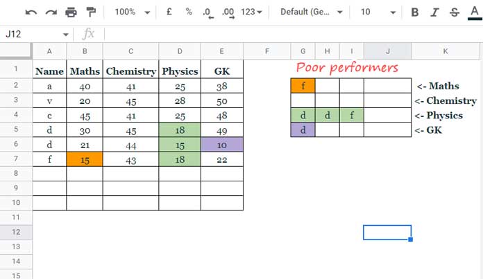
For example, we have a table with student names in the first column and their exam results in the adjoining few columns.
It’s in the order “Student Name,” “Maths,” “Chemistry,” “Physics,” and “General Knowledge.”
I want to filter the poor performers in each subject, starting with maths.
Using a Filter formula, we can filter the names of students who have scored less than 20 out of 50 in maths.
Transpose to move the layout from column to row. So we have the name of the poor performers in maths in one row.
When we drag the formula down, we need the name of the poor performers in chemistry in the next row.
How do we achieve this in Google Sheets?
The only way is to shift the criterion column from maths to chemistry when dragging down.
Note:-
Formula dragging down or right is not so standard after the introduction of Lambda functions in Google Sheets. They automate that process.
So, we can also get the desired Filter drag-down result using a Lambda formula.
I’ll leave that solution also at the end of this tutorial as a bonus. So here you go!
How to Shift a Column in a Filter Formula When Dragging It Down
We have the above data in cell range A1:E10, where A2:A10 is for names and B2:E10 is for marks in different subjects.
Usually, we can use the following FILTER formula to get the students’ names who have scored less than 20 in maths.
Formula # 1 (Step 1):
=ifna(filter($A$2:$A$10,B2:B10<20,B2:B10<>""))Copy-paste it to the right-hand side cell to get the name of the students in chemistry.
This act will shift the criteria column in the filter formula when dragging right, not down.
To shift the filter criteria column when dragging the filter formula down, you must make a few changes.
First and foremost, transpose the output using the TRANSPOSE function.
Formula # 2 (Step 2):
=transpose(ifna(filter($A$2:$A$10,B2:B10<20,B2:B10<>"")))Then replace B2:B10 with index($B$2:$E$10,0,row(A1), which will shift columns in the Filter formula when we drag it down.
Formula # 3 (Final Formula):
=transpose(ifna(filter($A$2:$A$10,index($B$2:$E$10,0,row(A1))<20,index($B$2:$E$10,0,row(A1))<>"")))You May Like: How to Use Google Sheets Index Function – Advanced Tips.
Automate Copy-Pasting Down Using the Bycol Lambda Function
Using the BYCOL function, we can automate the shift column in a filter formula without dragging it down.
You must empty the column range G2:J before inserting the following Bycol formula in cell G2.
Formula # 4 (Final Formula):
=transpose(bycol(B2:E10,lambda(c,ifna(filter($A$2:$A$10,c<20,c<>"")))))How does this formula be able to shift columns in each row in the filter row-by-row formula?
Let me walk you through the steps of it.
- Scroll up and take a look at Formula # 1 which is as follows
=ifna(filter($A$2:$A$10,B2:B10<20,B2:B10<>"")). - In that formula, here we replaced B2:B10 with the
c, which is the name of the column identifier B2:B10.=ifna(filter($A$2:$A$10,c<20,c<>"")). It will return an error value. You may ignore it. - Used the Bycol lambda function to group the array B2:E10 by columns by application of a LAMBDA function to each column which is like
=bycol(B2:E10,lambda(c,ifna(filter($A$2:$A$10,c<20,c<>"")))). - Then transposed the output and voila!