


")


")

")
")
 in Excel & Google Sheets")


Using Google Sheets Query with OR conditions across multiple columns can get messy. Writing out each column individually works for 2–3 columns, but it becomes unmanageable when you have 50 or more.
In this guide, you’ll learn a simple formula trick to handle several OR columns in Query without writing overly long and complex formulas.
This tutorial is part of the WHERE Clause in Google Sheets QUERY: Logical Conditions Explained hub, which covers all logical operators, comparisons, and condition-building patterns used in QUERY statements.
Why Multiple OR Columns Are Hard to Handle in Google Sheets Query
Suppose your data range in Sheet1 is A1:AX (50 columns).
You want to return names from column A if any column from F to AX contains a specific value.
For just a few columns, you might write:
=QUERY(Sheet1!A1:AX,
 "Select A where F='test' or G='test' or H='test' or I='test' or J='test'",
1)
But this becomes impossible to manage when you need to check 45+ columns.
Example: Attendance Data with OR Conditions Across Multiple Columns
| Name | Age | Class | Division | Teacher |
|---|---|---|---|---|
| Johnnie | 10 | 4 | A | Julio |
| Sarah | 11 | 4 | A | Julio |
| Micheal | 10 | 4 | A | Julio |
| Angela | 10 | 4 | B | Leland |
| Frank | 11 | 4 | B | Leland |
Columns F to AX contain attendance (P = Present, A = Absent) with headers as sequential dates.
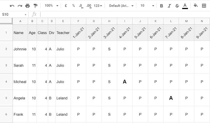
Goal: Return students who were absent (A) on any day.
Simplest Formula to Handle OR Conditions Across Multiple Columns in Google Sheets Query
Instead of writing many OR conditions, we’ll combine all columns into one helper column and check only that.
=ArrayFormula(QUERY(
  {Sheet1!A1:A, TRANSPOSE(QUERY(TRANSPOSE(Sheet1!F1:AX="A"),,9^9))},
  "SELECT Col1 WHERE Col2 contains 'TRUE'",
  1
))
Explanation:
Sheet1!F1:AX="A"converts the range into a TRUE/FALSE array, markingTRUEwhere a student was absent.TRANSPOSE(QUERY(TRANSPOSE(...),,9^9))combines all these columns into a single helper column (Col2), making it easier to search across multiple OR conditions.- For more details, see our related tutorial: A Flexible Array Formula for Joining Columns in Google Sheets.
{Sheet1!A1:A, …}pairs each student’s name with the helper column.QUERY(..., "SELECT Col1 WHERE Col2 contains 'TRUE'", 1)returns the names of students who have at least one absence.
Result: Micheal and Angela are correctly returned.
Note: This approach works with numeric data as well. We’ll demonstrate that using a numeric dataset later in the tutorial (see the last section).
Partial Matches (Matching Whole Words) in Google Sheets Query OR Conditions
If you want an approximate match—for example, matching just the first name in a column that contains full names—the previous TRUE/FALSE approach won’t work.
For instance, if you want to match “Arun” when the cell contains “Arun Varma”, you can use this formula:
=ArrayFormula(
  QUERY(
    {Sheet1!A1:A, " "&TRANSPOSE(QUERY(TRANSPOSE(Sheet1!F1:AX),,9^9))&" "},
    "SELECT Col1 WHERE Col2 contains ' Arun '",
    1
  )
)
Here’s what we changed:
- Removed the logical TRUE/FALSE test.
- Added spaces around both the criteria (
' Arun ') and the criteria range to ensure a whole-word match rather than matching substrings like “Arunima.”
Formula Explanation:
TRANSPOSE(QUERY(TRANSPOSE(Sheet1!F1:AX),,9^9))combines all columns into a single helper column (Col2), making it easier to search multiple columns at once." "&…&" "adds spaces around each value so thatCONTAINS ' Arun 'matches the full word only.{Sheet1!A1:A, …}pairs each student’s name with the helper column.QUERY(..., "SELECT Col1 WHERE Col2 contains ' Arun '", 1)returns the names where the first name matches exactly.
Numeric Example: Query Across Multiple OR Columns in Google Sheets
For numeric data, we can use the same approach as we did for text—applying a logical test that returns TRUE or FALSE. Here’s how it works:
Sample Dataset:
| Name | Math | Physics | Chemistry | Biology |
|---|---|---|---|---|
| Ben | 90 | 97 | 85 | 85 |
| Mike | 95 | 99 | 85 | 89 |
| John | 85 | 100 | 86 | 85 |
| Rose | 91 | 99 | 87 | 89 |
| Shika | 89 | 95 | 90 | 90 |
Goal: Filter students who scored ≥98 in any subject.
Formula:
=ArrayFormula(QUERY(
  {Sheet1!A1:A, TRANSPOSE(QUERY(TRANSPOSE(Sheet1!B1:E>=98),,9^9))},
  "SELECT Col1 WHERE Col2 contains 'TRUE'",
  1
))
Formula Explanation:
Sheet1!B1:E>=98converts the numeric range into a TRUE/FALSE array.TRANSPOSE(QUERY(TRANSPOSE(...),,9^9))combines all numeric columns into a single column of TRUE/FALSE values.{Sheet1!A1:A, …}pairs each student’s name with the combined column.QUERY(..., "SELECT Col1 WHERE Col2 contains 'TRUE'", 1)returns the names of students who scored 98 or higher in at least one subject.
This method is simple, avoids complicated formulas, and works perfectly for numeric comparisons across multiple columns.
Benefits of Using This Method Over Standard OR Conditions
- Avoids writing dozens of OR conditions manually
- Works with both text and numbers
- Supports exact or partial matching
- Keeps formulas shorter and easier to maintain