")
")


")


")

")
")
 in Excel & Google Sheets")


If you’ve ever needed to search for a specific value and sum up to that row in Google Sheets, this guide is for you. Whether you’re tracking totals until a certain task, date, or keyword appears, you can use a smart combination of formulas to do it dynamically. In this post, you’ll learn how to sum a column until a specific value is found in Google Sheets using functions like SUM, INDEX, and XMATCH.
This technique is especially useful in many situations. For example, consider a date column alongside an amount column. If you need to sum values up to a specific date, this method works perfectly.
In another scenario, imagine you’re reviewing a shipment log. You want to total the quantities until a particular product arrives — for instance, summing up values until the first occurrence of “Product X.”
Formula to Sum a Column Until a Specific Value is Found
=SUM(INDEX(C2:C, 1, 1):INDEX(C2:C, XMATCH(E2, B2:B), 1))Explanation of parameters:
E2: The lookup value (e.g., “Urgent Fix”)B2:B: The column where the value is searchedC2:C: The column to sum
Example: Add up working hours until a specific task appears
Here’s some sample data:
| Date | Task Name | Hours |
| 01/04/2025 | Email Responses | 1 |
| 01/04/2025 | Bug Fix #956 | 1.5 |
| 02/04/2025 | Standup Meeting | 0.5 |
| 02/04/2025 | Task ABC Review | 1 |
| 03/04/2025 | Urgent Fix | 3 |
| 03/04/2025 | Documentation | 1 |
Let’s sum the hours until “Urgent Fix” is reached:
=SUM(INDEX(C2:C, 1, 1):INDEX(C2:C, XMATCH(E2, B2:B), 1))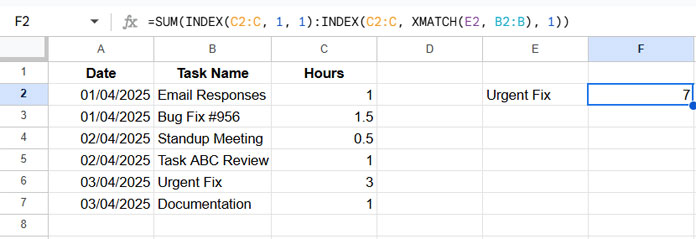
If you want to exclude “Urgent Fix” from the total, use this formula:
=SUM(INDEX(C2:C, 1, 1):INDEX(C2:C, XMATCH(E2, B2:B)-1, 1))How Does This Formula Sum a Column Until a Specific Value is Found in Google Sheets?
Let’s break it down:
=SUM(INDEX(C2:C, 1, 1):INDEX(C2:C, XMATCH(E2, B2:B), 1))INDEX(C2:C, 1, 1): From the rangeC2:C, return the first cell (i.e., C2)INDEX(C2:C, XMATCH(E2, B2:B), 1): From the same column, return the row where the value inE2appears inB2:B
This constructs a dynamic range from C2 to the row where the lookup value appears — e.g., C2:C6 — and sums it.
Alternative Formula to Sum a Column Until a Specific Value is Found
Here’s another way to create a dynamic range using ARRAY_CONSTRAIN:
=SUM(ARRAY_CONSTRAIN(C2:C, XMATCH(E2, B2:B), 1))This formula constrains the range C2:C to a number of rows equal to the result of XMATCH, and then sums it.
To exclude the row where the value is found, subtract 1:
=SUM(ARRAY_CONSTRAIN(C2:C, XMATCH(E2, B2:B)-1, 1))Related Use Cases
This technique is handy for many practical tasks:
- Sum until a specific date in financial logs
- Sum up working hours until a specific task appears
- Sum sales or inventory until a product is encountered
- Running totals until a milestone or keyword is reached
All of these are variations of the same powerful concept: Sum a Column Until a Specific Value is Found in Google Sheets — dynamically and efficiently.