How to Reset a Running Total by Month in Google Sheets

Google Sheets offers multiple ways to calculate a running total that resets each month. In this tutorial, you’ll learn the best approaches—both simple and efficient—so you can track monthly totals without breaking your workflow.

Table of Contents

Introduction

When working with datasets like sales, purchases, expenses, or income, you may often need a running total that restarts at the beginning of each month.

For example:

Monthly sales reports that shouldn’t carry over into the next month.
Expense tracking where each month’s budget resets.
Timesheets or project hours that need monthly totals.

A standard running total keeps adding values across all rows. With the right formula, however, you can make it reset automatically at every month change. Even better, the methods below can handle data spanning multiple years, ensuring that totals don’t overlap between different years.

By the end of this guide, you’ll know how to use both drag-down and array formulas to build flexible monthly running totals in Google Sheets that adapt as your dataset grows.

Sample Data

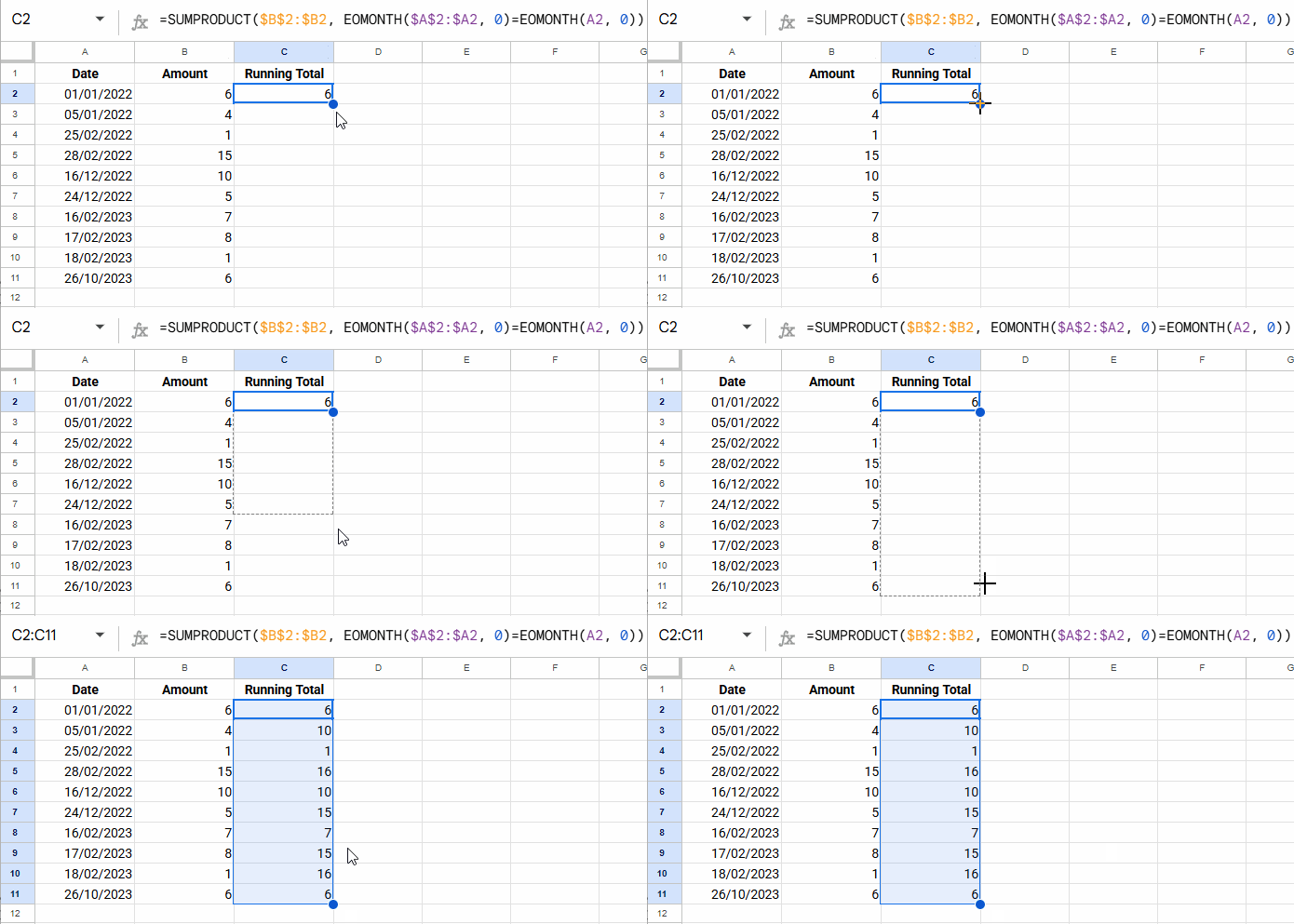
We’ll work with the following dataset in A1:B, where column A contains dates and column B contains amounts. The goal is to calculate a running total by month in column C.

Date	Amount
01/01/2022	6
05/01/2022	4
25/02/2022	1
28/02/2022	15
16/12/2022	10
24/12/2022	5
16/02/2023	7
17/02/2023	8
18/02/2023	1
26/10/2023	6

Formula to Reset a Running Total by Month (Sorted or Unsorted Dates)

Let’s begin with a drag-down formula that works whether your data is sorted or not.

=SUMPRODUCT($B$2:$B2, EOMONTH($A$2:$A2, 0)=EOMONTH(A2, 0))

Place this in C2 and drag it down.

GIF showing the SUMPRODUCT formula being entered in Google Sheets and dragged down to calculate a running total that resets by month

How it works:

EOMONTH($A$2:$A2, 0)=EOMONTH(A2, 0) → checks whether each row’s month (end of month date) matches the current row’s month.
This produces a TRUE/FALSE array (equivalent to 1/0).
SUMPRODUCT multiplies this array with the amounts in column B and sums them, giving the monthly running total.

✅ Using EOMONTH instead of MONTH ensures that the formula handles multiple years correctly.

Array Formula Version (No Dragging Required)

If you prefer a formula that spills automatically, use:

=MAP(A2:A, B2:B, LAMBDA(date_, amount_, IF(date_="",,
   SUMPRODUCT(B2:amount_, EOMONTH(A2:date_, 0)=EOMONTH(date_, 0))
)))

This uses the same logic as the drag-down version but applies it row by row with MAP and LAMBDA.
IF(date_="",,) ensures empty rows stay blank.

⚠️ Drawback: While it works in both sorted and unsorted datasets, this formula can become resource-intensive on very large datasets (thousands of rows).

Pros and Cons

Pros:

Works with both sorted and unsorted dates.
No helper columns needed.
Handles multiple years automatically.

Cons:

The array version (MAP + SUMPRODUCT) may slow down or freeze in very large datasets.

Formula to Reset a Running Total by Month (Sorted Dates)

If your dataset is sorted by date and especially if it’s very large, this SUMIF-based array formula is the better option:

=ArrayFormula(IF(LEN(A2:A), 
   SUMIF(ROW(A2:A), "<="&ROW(A2:A), B2:B) - 
   SUMIF(EOMONTH(A2:A, 0), "<"&EOMONTH(A2:A, 0), B2:B), 
))

How it works:

SUMIF(ROW(A2:A), "<="&ROW(A2:A), B2:B) → generates the standard cumulative sum.
SUMIF(EOMONTH(A2:A, 0), "<"&EOMONTH(A2:A, 0), B2:B) → calculates the cumulative sum up to the previous month.
Subtracting the second result from the first resets the total each month.

Pros and Cons

Pros:

Array formula (no dragging needed).
Efficient and scalable—ideal for very large datasets.
Correctly handles multiple years.

Cons:

Requires the date column to be sorted for accurate results.

Final Thoughts

Resetting a running total by month in Google Sheets is simple with the right formula:

Use SUMPRODUCT (drag-down or MAP version) if your data is small-to-medium and may not always be sorted.
Use the SUMIF-based array formula for large, sorted datasets where performance matters.

Both methods handle data spanning multiple years, ensuring that monthly totals reset correctly without overlap.

With these formulas, you can track monthly sales, expenses, or any time-based totals dynamically in Google Sheets—no manual resets required.