You can use SUMIF with BYROW in Google Sheets to sum the last column only when all the previous columns in a row meet the same condition. To make this work, the number of columns in the SUMIF range should match the total column, and the BYROW with COUNTIF takes care of that for you.

Here’s the formula:

=SUMIF(
  BYROW(B2:F, LAMBDA(r, COUNTIF(r, "Passed")=COLUMNS(r))),
  TRUE,
  G2:G
)

This checks each row, confirms whether every cell matches "Passed", and then sums the helper column accordingly.

Why Would You Need This?

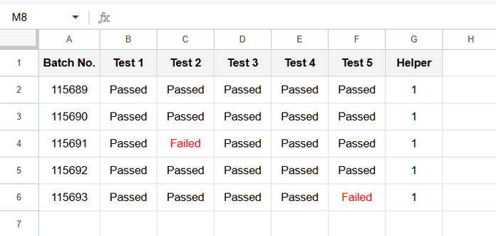
Imagine you’re running quality tests on a product batch. Each batch goes through five tests, and you only want to count the batches that passed all of them.

You could set up your data with:

• Column A: Batch number
• Columns B–F: Test results (Passed or Failed)
• Column G (Helper): Simply 1 to mark each batch

Then the formula above will give you the total number of batches that passed every test.

This isn’t limited to quality checks. The same idea works for:

• Attendance tracking: Count employees present on every day of the month.
• Survey responses: Sum participants who answered all questions positively.
• Task completion sheets: Total projects where every step was marked “Done.”

Example Dataset in Google Sheets

How the Formula Works to Sum the Last Column

=SUMIF(
  BYROW(B2:F, LAMBDA(r, COUNTIF(r, "Passed")=COLUMNS(r))),
  TRUE,
  G2:G
)

1. BYROW(B2:F, … ) → Processes each row of test results individually.
2. COUNTIF(r, "Passed")=COLUMNS(r) → Checks if the number of "Passed" values equals the number of tests (i.e., all passed).
3. Result of BYROW → Returns TRUE for rows where all tests are passed, FALSE otherwise.
4. SUMIF(..., TRUE, G2:G) → Sums the helper column only for the TRUE rows.

In the sample above, the formula returns 3, since only 3 batches passed every test.

When Each Row Should Have Identical Values

So far, we’ve used a fixed criterion like "Passed" for every column in a row. But what if you want to check whether all values in each row are identical, regardless of whether they’re "Passed", "OK", or something else?

That’s where this variation of the formula comes in:

=SUMIF(
  BYROW(B2:F, LAMBDA(r, COUNTIF(r, CHOOSEROWS(r, 1))=COLUMNS(r))),
  TRUE,
  G2:G
)

Here’s how it works:

• CHOOSEROWS(r, 1) picks the first cell in the row.
• COUNTIF(r, CHOOSEROWS(r, 1)) counts how many times that first value appears in the row.
• If that count equals the total number of columns (COLUMNS(r)), it means every value in that row matches the first one.
• Finally, SUMIF totals the helper column (G2:G) only for rows where all values are identical.

Example:

• If a row has 5 | 5 | 5 | 5 | 5 → ✅ counted.
• If another row has 2.30 | 2.30 | 2.30 | 2.30 | 2.30 → ✅ also counted.
• But if a row has 5 | 3 | 5 | 5 | 5 → ❌ not counted.

Where to Use This

This approach is useful when consistency matters more than a specific value. For example, imagine you’re testing different product batches (column A), each going through five quality checks. Since results can vary across products (like 5, 4.5, 2.3, etc.), you want to find out which batches had the same result across all tests.

In that case, this row-wise identical columns check ensures only those batches are counted in the total.

Key Takeaways

• You can use SUMIF with BYROW in Google Sheets to total a helper column only when the previous columns in each row meet certain conditions.
• With a fixed criterion (like "Passed"), the formula checks if every column in a row contains that exact value before summing the helper column.
• With the row-wise identical variation, the formula checks if all values in a row are the same — no matter if they’re 5, 4.5, or any other value.
• This approach is flexible and can be applied to scenarios like quality control tests, employee attendance tracking, or any dataset where you need to verify consistency across multiple columns.

Google Sheets Resources

• Filter Rows with Text in All Columns in Google Sheets
• Compare All Columns with Each Other for Duplicates in Google Sheets