In this tutorial, you’ll learn how to calculate a reverse running total—also known as a backward cumulative sum or reverse cumulative sum—in Google Sheets using both a regular formula and an array formula.

When your data is sorted from newest to oldest, a reverse running total can be more meaningful than a standard cumulative sum. This is especially useful when you want to see totals that accumulate from bottom to top—for instance, the remaining total from a point in time going backwards.

Example Use Case

Let’s use real-world data: wheat production in Australia from 2010 to 2019, sourced from Wikipedia.

In Google Sheets:

• Column A contains the years.
• Column B contains wheat production figures (in million metric tonnes).
• The data is sorted in descending order by year—from 2019 (newest) at the top to 2010 (oldest) at the bottom.

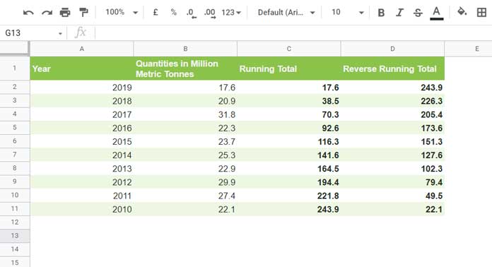
This setup is ideal for calculating a reverse cumulative sum in Google Sheets.

Understanding Reverse Running Total

A standard cumulative sum (or running total) adds values from top to bottom. In contrast, a reverse running total—or backward cumulative sum—adds values from bottom to top.

This helps answer questions like: “What was the total wheat production from this year onward?”

Non-Array Formula for Reverse Running Total

If you prefer a standard formula you can drag down, use this in cell D2:

=SUM($B$2:$B) - SUM($B$1:B1)

Explanation:

• SUM($B$2:$B): Calculates the total of all values in column B.
• SUM($B$1:B1): Sums everything above the current row (excluding the current row).
• The result is the reverse running total for each row.

Drag the formula down to apply it to the remaining rows.

This method works well for smaller or static datasets.

Array Formula for Reverse Running Total in Google Sheets

If you’d prefer a dynamic, drag-free solution, use this array formula in D2:

=ArrayFormula(IF(B2:B, SUMIF(ROW(B2:B), ">="&ROW(B2:B), B2:B), ))

This formula returns the reverse cumulative sum in Google Sheets for the range B2:B, automatically expanding as new rows are added.

Detailed Explanation:

• ROW(B2:B): Generates row numbers for each entry.
• ">="&ROW(B2:B): The condition used by SUMIF to include current and all subsequent rows.
• SUMIF(...): Sums the corresponding values in column B where the row number is greater than or equal to the current row.
• IF(B2:B, ..., ): Ensures blank rows are ignored.

This is a clean and scalable solution for reverse accumulation, especially useful in dynamic datasets.

Terminology Note

Whether you call it a reverse running total, a reverse cumulative sum, or a backward cumulative sum in Google Sheets, the logic and formula stay the same. These terms are often used interchangeably depending on the context or audience, but they all refer to accumulating values from bottom to top.

Related Resources

• Normal and Array Running Totals in Google Sheets
• Running Count in Google Sheets: Formula Examples
• How to Calculate Running Balance in Google Sheets (SUMIF and SCAN Solutions)
• Reverse Running Count Simplified in Google Sheets
• Running Max Values in Google Sheets (Array Formula Included)
• Find the Running Minimum Value in Google Sheets
• Calculating Running Average in Google Sheets (Array Formulas)