


I want to automatically change the cell reference of an Importrange formula when I drag it down. I mean, how do I get relative cell references in Importrange?
The ultimate goal is to import the next row when I copy an Importrange formula down and then import the next column when I copy the formula across.
As you may know, relative cell references change when you copy a formula down, up, right, or left.
By default Importrange function doesn’t support this as it takes range_string, which is a text.
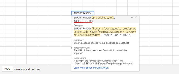
Syntax: IMPORTRANGE(spreadsheet_url, range_string)
I have the below Importrange formula in cell A1 in a blank sheet.
Formula 1:
=importrange("URL","Sheet1!A2:F2")Note:- Replace the URL with the full URL of your Google Sheets file. I mean the URL that starts with https://, not the Spreadsheet ID (GID) only.
As you can see, when I drag this Importrange formula, it copies the same formula. The cell reference doesn’t become A3:F3.
How to Get Relative Cell Reference in Importrange by Replacing Range_String
We can replace range_string with a combo formula to bring dynamism to range_string. It makes dynamic cell reference possible in Importrange.
We will use four functions in the combo formula. They are Address, Row, Column, and Join.
Let me show you how to develop that combo formula to bring relative cell reference reality in the Google Sheets Importrange function.
Use it and get the next row or column data in the Importrange.
Dynamic Cell Reference Using Address, Row, and Column Combo in Importrange
In the above example, I want to import the row range Sheet1!A2:F2, and when I drag it down, I want to change this reference to Sheet1!A3:F3, the next row.
Here is how to generate a relative cell reference range to use in Importrange.
Steps
1. Insert the following formula in a blank cell and see the output. The result would be Sheet1!$A$2.
=address(row(A2),column(A2),,,"Sheet1")Change “Sheet1” in the above formula with the sheet name of your source sheet to import.
2. The following formula returns the cell reference $F$2.
=address(row(F2),column(F2))3. Combine both the above formulas as below using the Join function.
=join(":",address(row(A2),column(A2),,,"Sheet1"),address(row(F2),column(F2)))Output: Sheet1!$A$2:$F$2
4. Now you can replace the range_string, i.e., “Sheet1!A2
Formula 2:
=importrange("URL",join(":",address(row(A2),column(A2),,,"Sheet1"),address(row(F2),column(F2))))
When you copy this formula down, it will import the data from A3:F3, i.e., the next row of data.
Can We Copy It Across the Row?
You can copy it across the row when importing a single column.
For example, I am importing A2:A10 in cell A1. When I copy this Importrange form A1 to A2, I want to import B2:B10.
Then the formula in the above third step will be as follows.
=join(":",address(row(A2),column(A2),,,"Sheet1"),address(row(A10),column(A10)))It will import the next column’s data when copying it across.
Follow this approach to get relative cell references in Importrange in Google Sheets. Thanks for the stay. Enjoy!
Related: How to Freeze a Cell in Importrange in Google Sheets.
Thank you so much! This was a super helpful way to show how to do it! It saved me a lot of time 🙂
It worked! I used the new formula, and it’s working! Thank you so much. I really appreciate it.
Hi Prashanth,
In one row, I am trying to pull data from my source document and sheet.
My formula looks like this for cell 1:
=IMPORTRANGE("https://URL", join(":",address(row(H198),column(H198),,,"Sheet1")))As I drag the cells across, the columns change, so it looks like this for cell 2:
=IMPORTRANGE("https://URL", join(":",address(row(I198),column(I198),,,"Sheet1")))However, I am trying to find a way that the column remains static and the row number change:
=IMPORTRANGE("https://URL", join(":",address(row(H199),column(H199),,,"Sheet1")))Is there a way to do this?
Thank you for responding so quickly
Hi, Angela,
Thanks for the explanation.
You are dragging the formula across.
You want the column to remain static. So use
8instead ofcolumn(H198), which represents column H.Since you want the row to change from 198 to 199, 200 and so on, use
column(A1)+197instead ofrow(H198).So the formula will be
=IMPORTRANGE("https://URL",join(":",address(column(A1)+197,8,,,"Sheet1")))Note:- You can instead import and transpose the required ranges as below.
=TRANSPOSE(IMPORTRANGE("https://URL","Sheet1!H198:H202"))Hi Prasanth,
Thank you for this.
I want the column to stay the same, but only change the row # with a copy and drag.
What would the formula look like?
Hi, Angela,
Please clarify. If you drag the formula down, only the row number changes.
Hi,
Thank you. It was super useful and thoughtful 🙂
Thanks! After a LOT of searching I finally found this page and got my problem solved, so thank you so much! 🙂
However I do have a question: If I add (or remove) a row above the formula in the final sheet, then the formula also “adds” (or “removes”) a row, leading to the wrong info being displayed. Is there a way around this?
Nope! That’s how relative cell reference works.
Ok, I’ll just have to plan the final sheet very carefully then. Thanks again for the info and for your quick reply.