


You have multiple tasks and multiple people. Here’s a fun way to randomly assign a task to a random person in Google Sheets.
The fun element lies in the automation of the random task assignment. Here’s how it works:
The top row contains tasks, while the first column contains names (students, employees, or your friends’ names), with the grid between them filled with checkboxes.
The free template initially assigns a random task to a random person. It does this by highlighting an unchecked tick box randomly.
Once you tick that box, it randomly highlights another tick box, and this process continues until you tick all the checkboxes.
You can use this interactive Random Task Assigner template straight out of the box. However, I strongly suggest following the step-by-step instructions below to help you adjust the template to meet your specific requirements.
Free Random Task Assignment Template for Google Sheets and How to Use It
You can preview and obtain a copy of this free Random Task Assigner template by clicking the button below.
The template is configured for 20 tasks and 20 people, but feel free to adjust the number of columns (tasks) and rows (names) as needed.
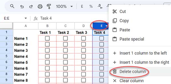
To remove a column, simply right-click on the column letter at the top and select “Delete column” from the context menu.
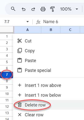
To delete a row, right-click on the row number on the left and choose “Delete row” from the context menu.
If you have additional tasks or names, insert rows or columns within the grid, avoiding the beginning or end. You can access these options by right-clicking the row number or column letter and selecting the relevant options from the context menu.
Replace ‘Task 1’, ‘Task 2’, etc. with your specific tasks and ‘Name 1’, ‘Name 2’, etc. with actual names.
Once you’ve made your adjustments, click the drop-down menu (currently located in cell V2) and select “Yes” to initiate the highlighting process. Do not select “No” afterward.
Click on the checkbox in the highlighted cell (representing the randomly assigned task in the grid). This will prompt the highlighting of another task. Continue this process until you have checked all cells.
What happens if I tick a checkbox that isn’t highlighted?
You can tick one or more checkboxes to prevent the template from highlighting them. For instance, if you wish to exclude Task 10 from the assignment, select cells K2:K21 and press the spacebar. This action ticks all the checkboxes in that range, indicating that these tasks are not to be assigned to anyone.
Important
If you encounter any issues with the Random Task Assigner template not responding to user interaction, you can resolve it by following these steps:
- Copy the formula located in cell W2.
- Delete the formula in cell W2.
- Paste the copied formula back into cell W2.
This should ensure that the template functions properly.
The Key Formula Used in the Random Task Assigner and Its Role
The template incorporates a formula within a cell and another formula within conditional formatting.
The pivotal formula, found in cell W2, is as follows:
=LAMBDA(cell, IF(V2="Yes", cell, ))(
   ArrayFormula(
      LET(
         grid, B2:U21,
         test,
         TOCOL(IF(grid=TRUE, ,ADDRESS(ROW(grid), COLUMN(grid))), 1),
         IFERROR(SORTN(test, 1, 0, RANDARRAY(COUNTA(test)), 1))
      )
   )
)
What role does this formula play in assigning a random task to a random person?
This formula returns a random cell address from within the grid while ensuring that it excludes cells that have already been ticked.
Here’s a breakdown of the formula in its simplest form:
Step 1:
LET assigns the name ‘grid’ to the range B2:U21, which contains the tick boxes.
Step 2:
Generate the addresses of unticked cells within the ‘grid’ using the formula:
TOCOL(IF(grid=TRUE, ,ADDRESS(ROW(grid), COLUMN(grid))), 1)The result is assigned to the variable ‘test’.
Step 3:
Sort the cell addresses returned in the previous step in ascending order based on randomly generated numbers by the formula:
IFERROR(SORTN(test, 1, 0, RANDARRAY(COUNTA(test)), 1))This formula returns one random cell address, as the SORTN function returns sorted ‘n’ values, where ‘n’ in this case is 1.”
Highlighting a Cell in the Grid Matching the Cell Address
We have a random cell address representing the random task to assign. We’ll employ conditional formatting to highlight the corresponding cell within the grid.
I’ve applied the following rule, which tests whether each cell address in the grid is equal to the cell address returned by the key formula in cell W2:
=CELL("address", B2)=$W$2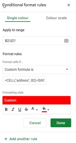
If a match occurs, the cell highlights.
Resources
Here are some related topics in Google Sheets:
- How to Pick a Random Name in Google Sheets (Does Not Refresh)
- Google Sheets: Macro-Based Random Name Picker
- How to Randomly Select N Numbers from a Column in Google Sheets
- How to Randomly Extract a Certain Percentage of the Rows in Google Sheets
- How to Generate Odd or Even Random Numbers in Google Sheets
- Pick Random Values Based on Conditions in Google Sheets