This tutorial isn’t just about how to use the QUERY function to combine columns in Google Sheets—although that’s certainly part of it. The main focus here is on how to insert or add separators (also known as delimiters) when combining column values using the QUERY function.

We often use the QUERY function to concatenate columns in Google Sheets. However, it’s not the only way—using the & operator with ARRAYFORMULA is another simple method.

✅ Ampersand to Combine Columns B to E (Formula #1)

=ARRAYFORMULA(B:B & " " & C:C & " " & D:D & " " & E:E)

While this method works, it has a limitation: when combining many columns, using the ampersand (&) becomes inefficient because each column must be referenced individually.

This is where using a query to combine columns and adding separators becomes a better alternative. The QUERY function allows you to refer to an entire range of columns, which simplifies the formula and makes it easier to manage.

If you choose not to use QUERY, another modern approach is to use BYROW with a custom LAMBDA function. It’s more flexible and compact, though it can be resource-intensive on larger datasets. Here’s an example using BYROW.

✅ Formula #2

=BYROW(B:E, LAMBDA(row, JOIN(" ", row)))

However, as mentioned earlier, the main focus of this post is to show how to add separators or delimiters when using a query to combine columns in Google Sheets.

Using QUERY Header Clause to Combine Columns

Let’s start with a basic example of how to combine columns using QUERY in Google Sheets.

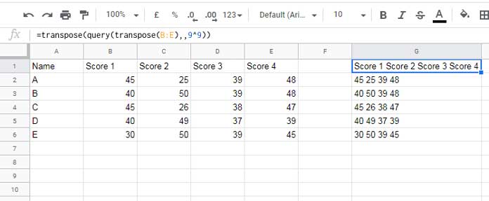
The formula below, entered in cell G1, combines columns B, C, D, and E. It uses the QUERY function to merge them row-wise. While the output appears to have space separators, no space is explicitly added—QUERY simply joins the values directly.

✅ Query to Combine Columns B to E (Formula #3)

=TRANSPOSE(QUERY(TRANSPOSE(B:E),,9^9))

This technique is explained in more detail here: A Flexible Array Formula for Joining Columns in Google Sheets

How This Works (Quick Recap)

• TRANSPOSE(B:E) flips the column data into rows.
• QUERY(..., , 9^9) treats all rows as headers and combines the values.
• The final TRANSPOSE(...) flips the result back into a single column of merged values.

We use TRANSPOSE twice because the QUERY function combines data across rows—not columns. This double-transpose trick allows us to combine columns using QUERY effectively.

Query to Combine Columns and Adding Delimiters

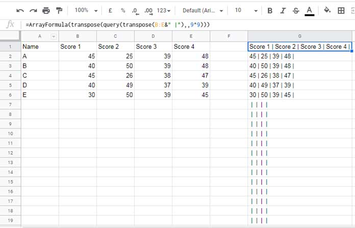
To insert a separator—like a pipe (|)—between the values, we first add the delimiter to the original data range.

✅ Formula #4

=ArrayFormula(TRANSPOSE(QUERY(TRANSPOSE(B:E&" |"),,9^9)))

We add a pipe preceded by a space to match the implicit spacing added by QUERY. Don’t add a space after the pipe, as that would introduce extra spacing in the final result.

This creates a new column of combined values, but also introduces a few problems.

Common Issues with Delimiters in Combined Columns

1. Extra delimiters at the end of each row.
   Since there are 4 columns, the result has 4 delimiters—even if some values are blank.
2. Delimiters in blank rows.
   QUERY does not automatically filter out rows without data.
3. Extra delimiters between values if some cells are empty.
   For example, if column C is empty in a row, you’ll see double pipes like "value1 | | value3".

Clean Up Extra Separators in the Output

To clean up the result, we can wrap the QUERY function inside two REGEXREPLACE functions. This allows us to:

• Remove repeated delimiters (| |)
• Trim trailing delimiters at the end of the line

✅ Final Formula (Cleaned Output)

=ArrayFormula(
   REGEXREPLACE(
      REGEXREPLACE(
         TRANSPOSE(QUERY(TRANSPOSE(B:E&" |"),,9^9)), "\s*\|\s*(\|\s*)*", " | "
      ), " \|\s*$", ""
   )
)

How it Works:

• The first REGEXREPLACE:
  • "\s*\|\s*(\|\s*)*" removes repeated or empty delimiters like | | |.
• The second REGEXREPLACE:
  • "\s*\|\s*$" removes the trailing delimiter at the end of each line.

This gives us clean, readable, and properly separated combined values.

Summary

If you’re looking for a query to combine columns and add separators or a query to combine columns and add delimiters, using QUERY along with TRANSPOSE, ARRAYFORMULA, and REGEXREPLACE provides a powerful and dynamic solution in Google Sheets.

Unlike manual approaches with &, this method handles large column ranges more efficiently and gives you full control over the output format.

Related Resources

• How to Remove Extra Delimiters in Google Sheets
• Remove Repeated Characters from the End of Strings in Google Sheets
• Split Numbers from Text Without Delimiters in Google Sheets
• Insert Delimiter into a Text After N or Every N Character in Google Sheets
• Substitute Nth Match of a Delimiter from the End of a String in Google Sheets
• Extract Last N Values from a Delimiter Separated String in Google Sheets
• How to Replace Every Nth Delimiter in Google Sheets