The Proper function is not a supported scalar function in Query. Then how to use the Proper function in Google Sheets Query?
I’ll explain that this time with two examples below.
Google Sheets Query supports upper() and lower() scalar functions, not proper().
To learn how to use the upper() and lower() scalar functions in Query, please check my tutorial linked below.
Must Read: How to Apply Bulk Change Case in Google Sheets Using Query Function.
The Proper function is available in Google Sheets but not in Query. You can use it as below.
=proper("info inspired")Result: “Info Inspired”
The syntax is like this.
PROPER(text_to_capitalize)The Proper() function in Google Sheets will change the case of the first letter in each word to capital and the rest to lower. Now, back to how to use the Proper function in Query with a workaround.
Must Read: Change Text to Upper, Lower, and Sentence Case.
Proper Function in Google Sheets Query
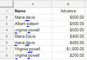
In the below sample data, the names are not grammatically correct. We must enter people’s names in the proper case (there are exceptions, though).
But our issue is different. The same name appears more than once in non-identical letter cases.

It would affect grouping and total in Google Sheets Query.
The solution is to use lower() or upper() scalar functions in the Select clause as below.
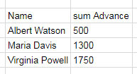
=query(A1:B8,"Select upper(A), sum(B) group by upper(A)",1)If you use the Query as below, the output won’t be correct.
=query(A1:B8,"Select A, sum(B) group by A",1)I have demonstrated the same in the below screenshot.

But if you want the grouped output in the proper() case, the formula will be as follows.
=ArrayFormula(query({proper(A1:A8),B1:B8},"Select Col1, sum(Col2) group by Col1",1))The above formula is an example of how to use the Proper function in Google Sheets Query.
In that formula, I have created a virtual range containing proper names in column A and the amount in column B.
For that, in addition to the Proper function, I have used the Curly Brackets and ArrayFormula.

Note:- Instead of the Curly Brackets, we can use HSTACK also. In that case, you may replace {proper(A1:A8),B1:B8} with hstack(proper(A1:A8),B1:B8).
There is one more scenario.
If you use a Query just for filtering a table, or you have an output of a Query containing only text strings, then you can wrap the Query with the Proper() function as below.
In my sample data (I am skipping the screenshot), column A contains employee names in mixed-case letters.
The contents in column B are just the letters A and P: A for “absent,” and P represents “present.”
That means both columns contain text strings.
The below Query formula filters all employees who are present.
=query(A1:B12,"Select A where B='P'",1)To make the names in Proper case, wrap the formula with the proper() function and use ArrayFormula.
=ArrayFormula(proper(query(A1:B12,"Select A where B='P'",1)))Related: How to Format Date, Time, and Number in Google Sheets Query.


Thank you, Prashanth. This page helped me to debug;
=ArrayFormula(query({proper(expertregistration20190925!$B1:$B),expertregistration20190925!$C1:$O},"select Col1,
lower(Col4) where Col14='Project'",1))
Many thanks.
Hi, Frank,
Thanks for your feedback!