The PERCENTRANK functions in Google Sheets return the percentile of a value, which represents its relative standing within a dataset.
Google Sheets provides three functions to calculate percentile ranks:
- PERCENTRANK
- PERCENTRANK.INC
- PERCENTRANK.EXC
How do these functions differ? Don’t worry—I’ll explain each one in detail with examples.
How to Use PERCENTRANK Functions in Google Sheets
1. PERCENTRANK
The PERCENTRANK function calculates the percentile of a given value within a dataset. It returns a decimal between 0 and 1, where:
- 0 means the value is the smallest in the dataset.
- 1 means the value is the largest.
- A decimal (e.g., 0.75) indicates that the value is higher than 75% of the dataset.
Syntax:
PERCENTRANK(data, value, [significant_digits])- data – The range of values in the dataset.
- value – The specific value whose percentile needs to be determined.
- significant_digits (optional) – The number of decimal places to include in the result (default is 3).
Note: The default value for significant_digits is 3, meaning results are rounded to three decimal places (e.g., 0.678). If you specify 0 or a negative number, Google Sheets will default to 3 decimal places.
Example of PERCENTRANK in Google Sheets
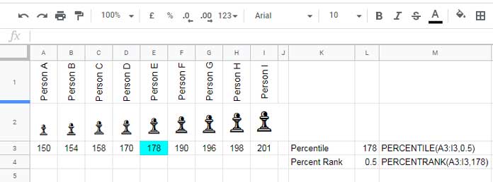
In the dataset below, we have the heights of 9 people (cells A3:I3).

To find the percentile of 178 cm, use:
=PERCENTRANK(A3:I3, 178)This returns 0.5 (50%), meaning 178 cm is higher than 50% of the dataset.
2. PERCENTRANK.INC
The PERCENTRANK.INC function works exactly like PERCENTRANK, as both include 0 and 1 in their possible results. You can use them interchangeably.
Syntax:
PERCENTRANK.INC(data, value, [significant_digits])Key Notes:
- PERCENTRANK and PERCENTRANK.INC return the same results.
- The smallest value in the dataset gets a percentile of 0.
- The largest value gets a percentile of 1.
Example:
If we apply the PERCENTRANK.INC function to the same dataset as before:
=PERCENTRANK.INC(A3:I3, 178)It returns 0.5 (50%), just like PERCENTRANK.
3. PERCENTRANK.EXC
The PERCENTRANK.EXC function is slightly different. It excludes 0 and 1 from its possible results.
- This means the smallest value won’t have a percentile of 0, and the largest value won’t have a percentile of 1.
- Instead, values are ranked between 0 and 1.
Syntax:
PERCENTRANK.EXC(data, value, [significant_digits])Key Difference:
- PERCENTRANK.INC (or PERCENTRANK) → Includes 0 and 1 (smallest value gets 0, largest gets 1).
- PERCENTRANK.EXC → Excludes 0 and 1 (smallest and largest values get a percentile slightly above 0 and below 1, respectively).
Example:
Using =PERCENTRANK.EXC(A3:I3, 190) and =PERCENTRANK.INC(A3:I3, 190) may return slightly different values because PERCENTRANK.EXC adjusts the percentile range by excluding 0 and 1, whereas PERCENTRANK.INC includes them.
PERCENTILE vs. PERCENTRANK in Google Sheets
Many users confuse PERCENTILE with PERCENTRANK, but they serve different purposes:
- PERCENTILE function returns the value at a given percentile.
- Example:
=PERCENTILE(A2:I2, 0.5)returns the value at the 50th percentile.
- Example:
- PERCENTRANK function returns the percentile of a given value.
- Example:
=PERCENTRANK(A2:I2, 178)returns 0.5, meaning 178 cm is at the 50th percentile.
- Example:
Summary of Differences:
| Function | Returns | Example Usage |
| PERCENTILE | The value at a given percentile | =PERCENTILE(A2:I2, 0.5) → Returns 178 cm (the median value) |
| PERCENTRANK | The percentile of a value in the dataset | =PERCENTRANK(A2:I2, 178) → Returns 0.5 (50%) |
Conclusion
The PERCENTRANK functions in Google Sheets help determine how a value compares to others in a dataset.
- PERCENTRANK and PERCENTRANK.INC are identical and include 0 and 1.
- PERCENTRANK.EXC excludes 0 and 1, giving slightly different results.
- PERCENTILE is different—it returns a value rather than a percentile.
I hope this guide clarifies everything! Let me know if you have any questions.


