


")


")

")
")
 in Excel & Google Sheets")


I’m confident you’ll find these percentile rank wise conditional formatting tips useful. You can easily apply them to your day-to-day Google Sheets tasks. Here’s an example of how percentile rank wise conditional formatting works.
In a written test, if your percentile rank is 0.75, it means you performed better than 75% of the other applicants who took the test. Simply put, you outperformed 75% of the test-takers.
How to Highlight the Top 25% of Scores?
A custom conditional formatting formula using the PERCENTILE or PERCENTRANK function can highlight values that fall within specific percentile ranges—such as between the 75th percentile and 100th percentile, i.e., the top 25% of scores.
Additionally, you can highlight the kth percentile value, whether or not it is an exact match in the dataset.
Percentile Rank Wise Conditional Formatting: Highlighting Data Within Adjustable Ranges
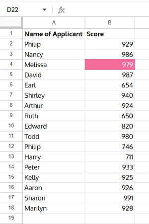
Sample Data:
| Name of Applicant | Score |
| Philip | 929 |
| Nancy | 986 |
| Melissa | 979 |
| David | 987 |
| Earl | 654 |
| Shirley | 940 |
| Arthur | 924 |
| Ruth | 650 |
| Edward | 820 |
| Todd | 980 |
| Philip | 746 |
| Harry | 711 |
| Peter | 933 |
| Kelly | 925 |
| Aaron | 926 |
| Sharon | 991 |
| Marilyn | 928 |
How to Highlight the Top 25% of Scores?
Steps:
1. Select A2:B18 (to highlight both columns) or B2:B18 (to highlight only the “Score” column).
2. Click on Format > Conditional Formatting.
3. Under “Format Rules,” select “Custom formula is”.
4. Enter the following formula:
=AND($B2>PERCENTILE($B$2:$B$18, 0.75), $B2<=PERCENTILE($B$2:$B$18, 1))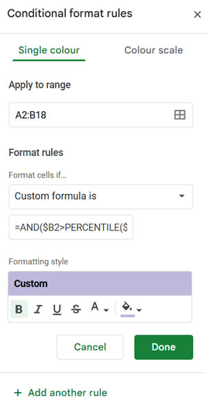
5. Choose a Fill Color and click Done.
This will highlight the top 25% of rows based on scores in the dataset.
How Does This Formula Work?
- The PERCENTILE function calculates the 75th and 100th percentile values.
- The AND function checks if both conditions are TRUE.
- The logical conditions are:
$B2 > PERCENTILE($B$2:$B$18, 0.75)– Checks if the score is above the 75th percentile.$B2 <= PERCENTILE($B$2:$B$18, 1)– Ensures the score is within the top 100% percentile range.
Alternative Method Using PERCENTRANK
Instead of PERCENTILE, you can use the PERCENTRANK function:
=ISBETWEEN(PERCENTRANK($B$2:$B$18, $B2), 0.75, 1, FALSE, TRUE)Explanation:
- PERCENTRANK returns the percentile rank of each value in column B.
- ISBETWEEN checks whether the percentile rank falls between 0.75 (exclusive) and 1 (inclusive).
This is another method of applying percentile rank wise conditional formatting in Google Sheets.
How to Highlight Only the Nth Percentile Value?
Sounds simple, right? Yes! But there’s a small technical challenge we need to address. Let’s dive deeper.
Highlighting the Exact Nth Percentile Value
Compared to percentile rank wise conditional formatting, highlighting just the nth percentile is much simpler.
Suppose you want to highlight the 75th percentile in the dataset.
Formula to get the 75th percentile value:
=PERCENTILE($B$2:$B$18, 0.75)Conditional Formatting Formula:
- Go to Format > Conditional formatting.
- Apply to range: B2:B18.
- Use this custom formula:
=$B2=PERCENTILE($B$2:$B$18, 0.75) - Set a fill color and click Done.
This formula highlights 979 in cell B4. However, there’s a catch!
Why Doesn’t This Work Every Time?
Sometimes, the percentile value calculated by the PERCENTILE function does not exist in the dataset. This happens because Google Sheets interpolates values to determine percentile positions.
Example:
=PERCENTILE($B$2:$B$18, 0.7)This returns 947.8, which is not in the dataset.
Solution: Matching the Closest Percentile Value
To highlight the nearest percentile value (even if it’s not an exact match), use XLOOKUP:
=$B2=XLOOKUP(PERCENTILE($B$2:$B$18, 0.7), $B$2:$B$18, $B$2:$B$18, , -1)How This Works:
- XLOOKUP finds the closest value in the dataset that is ≤ the calculated percentile value.
- The formula ensures conditional formatting applies correctly, even when the percentile isn’t an exact match.
Conclusion
That’s all about percentile rank wise conditional formatting in Google Sheets!
You now know how to:
- Highlight the top percentile ranks dynamically.
- Highlight values within a percentile range.
- Highlight the exact nth percentile value, even when it’s not a member of the dataset.
Try these methods and make your Google Sheets more insightful and visually appealing!