The PERCENTILE function returns the value at a specified percentile within a dataset in Google Sheets. The percentile is expressed as a decimal between 0 and 1, inclusive.

Before using the built-in function, let’s first understand how to find the value at a given percentile manually.

Manually Finding the Value at a Given Percentile in Google Sheets

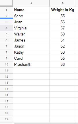
For example, consider the weights of a group of nine people.

To determine the value at a given percentile manually, follow these steps:

Step 1: Sort the Data in Ascending Order

We have the names of nine people in A2:A10 and their weights (in kg) in B2:B10.

First, arrange the data in ascending order based on weight (if not already sorted):

1. Select A2:B10
2. Click Data > Sort range > Advanced range sorting options
3. Select Sort by Column B and click Sort

Step 2: Calculate the Index Number

The index number is calculated using the formula:

Index=(Percentile)×(Count of values−1)+1

Since the dataset in B2:B10 represents 100%, we find the k-th percentile, where k is any percentage between 0 and 100.

To calculate the index position for the 75th percentile:

=75% * (COUNT(B2:B10)-1)+1  // Returns 7

• 75% represents the 75th percentile.
• COUNT(B2:B10) returns 9, the total number of data points.
• Subtracting 1 accounts for the fact that percentiles divide a dataset into intervals, not data points.
• Adding 1 adjusts for Google Sheets’ 1-based indexing.

Step 3: Find the Value at the Index

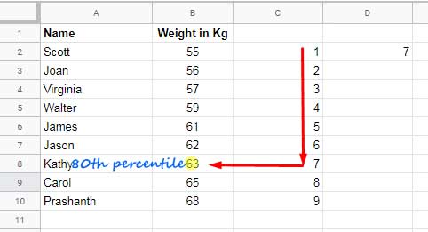
To easily identify index positions, generate a sequence from 1 to 9 in C2:C10:

=SEQUENCE(9)

Now, find the 7th value in column B. That value is 63, meaning 75% of people weigh less than Kathy (63 kg).

Handling Decimal Index Values (Interpolation)

If the index is not a whole number, interpolation is required.

For example, calculating the 80th percentile:

=80% * (COUNT(B2:B10)-1)+1  // Returns 7.4

• The 7th and 8th values in the dataset are 63 and 65, respectively.
• To interpolate:

=63 + (0.4 * (65 - 63))  // Returns 63.8

Where 0.4 is the decimal part of the index.

Thus, the 80th percentile value is 63.8.

Using the PERCENTILE Function in Google Sheets

The PERCENTILE function simplifies this process by directly returning the value at a specified percentile.

Syntax:

PERCENTILE(data, percentile)

Arguments:

• data – The range containing numeric values.
• percentile – The percentile (between 0 and 1) whose corresponding value will be returned.

Example:

Instead of manually calculating the 80th percentile, use:

=PERCENTILE(B2:B10, 0.8)

Key Insight:

The PERCENTILE function divides the dataset into two parts:

• Values that fall below the percentile threshold
• Values that fall above the percentile threshold

Alternative Percentile Functions in Google Sheets

Google Sheets provides two additional functions for calculating percentiles:

1. PERCENTILE.INC

• Same as PERCENTILE; both functions return identical results.
• You can use either interchangeably.

2. PERCENTILE.EXC

• Does not accept 0 (0%) or 1 (100%) as valid percentile inputs.
• Requires the percentile to be strictly between 0 and 1 (i.e., 0 < percentile < 1).

Example:

=PERCENTILE.EXC(B2:B10, 0)  // Returns #NUM! error  
=PERCENTILE.INC(B2:B10, 0)  //  Returns 55  
=PERCENTILE(B2:B10, 0)  //  Returns 55  

Unlike PERCENTILE.INC and PERCENTILE, which allow percentiles of 0 and 1, PERCENTILE.EXC only works with values strictly between 0 and 1.

Conclusion

The PERCENTILE function in Google Sheets is a powerful tool for determining values at specific percentile ranks within a dataset. Whether you use PERCENTILE, PERCENTILE.INC, or PERCENTILE.EXC, these functions eliminate the need for sorting and manual calculations.

Additional Resources

• PERCENTRANK Functions in Google Sheets
• Percentile Rank Wise Conditional Formatting in Google Sheets
• Calculating Percentile for Each Group in Google Sheets
• Get Top N% Scores Per Group in Google Sheets Dynamically