


")


")

")
")
 in Excel & Google Sheets")


In a nested VLOOKUP formula in Google Sheets, you place one VLOOKUP inside another. The inner VLOOKUP acts as the search_key for the outer VLOOKUP.
When using nested VLOOKUPs, the most common issue you’ll face is with column order.
I know—it’s not immediately clear. Let me explain.
You’ll typically work with two tables in a nested VLOOKUP setup. If the value returned by the inner VLOOKUP isn’t found in the first column of the outer VLOOKUP’s lookup range, the formula will return a #N/A error.
So, how do you work around that?
This post covers the issue and the solution. Let’s look at how to nest two VLOOKUP formulas in Google Sheets properly.
Sample Data
Note: You can click the button below to copy my sample Google Sheet and follow along.
We have two tables:
- Table 1: Driver name and their assigned vehicle number
- Table 2: Vehicle number and fuel consumption in gallons
Table 1 – Vehicle and Driver (Range: Sheet1!B2:C7)
| Driver | Vehicle Number |
|---|---|
| Albert | 96D123 |
| Paul | 96A154 |
| Justin | 96F452 |
| Samuel | 95A100 |
| James | 95F011 |
Table 2 – Vehicle and Fuel Consumption (Range: Sheet1!E2:F7)
| Vehicle Number | Fuel Consumption (gal) |
|---|---|
| 96D123 | 743.00 |
| 96A154 | 783.00 |
| 96F452 | 373.00 |
| 95A100 | 410.00 |
| 95F011 | 461.00 |
You might wonder: Do the vehicle numbers in both tables need to be in the same order?
The answer is no. In this case, the order was preserved only because I copy-pasted the data for simplicity.
Problem to Solve Using Nested VLOOKUP in Google Sheets
Let’s say you want to find the fuel consumption for the vehicle driven by Paul.
That means:
- Lookup “Paul” in Table 1 to get the vehicle number.
- Use that vehicle number to look up the fuel consumption in Table 2.
This could be useful, for example, if you want to calculate how much fuel reimbursement Paul is owed.
Step-by-Step: Nested VLOOKUP in Google Sheets
Step 1: VLOOKUP to Get the Vehicle Number
This formula returns the vehicle number assigned to Paul:
=VLOOKUP("Paul", B3:C7, 2, 0)Or, if “Paul” is entered in cell H3, you can use:
=VLOOKUP(H3, B3:C7, 2, 0)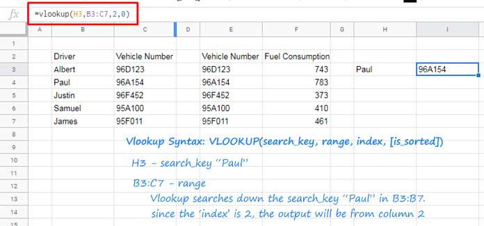
Step 2: Nest the VLOOKUP to Find Fuel Consumption
Now that we know the vehicle number (96A154), we can use it as the search key in another VLOOKUP.
Here’s the nested formula:
=VLOOKUP(VLOOKUP(H3, B3:C7, 2, 0), E3:F7, 2, 0)Result: 783.00
The inner VLOOKUP fetches the vehicle number for Paul, and the outer VLOOKUP uses that number to find the fuel consumption from Table 2.
Nested VLOOKUP Limitation: First Column Only
As mentioned earlier, VLOOKUP only searches in the first column of the lookup range. This becomes an issue when your search key isn’t in the first column.
You can solve this in two ways:
- Use XLOOKUP instead, which doesn’t require the search key to be in the first column—since it uses separate search and return ranges instead of a single lookup range.
- Rearrange the columns virtually using the HSTACK function or curly braces
{}.
Let’s walk through an example that involves reordering columns for nested VLOOKUP to work.
Nested VLOOKUP: Search Column Other Than First Column
Imagine two new tables on Sheet2:
- Table 1 (Range A2:B): Employee ID and Name
- Table 2 (Range D3:H): Sales volumes from Jan to Apr, with Employee ID in the last column
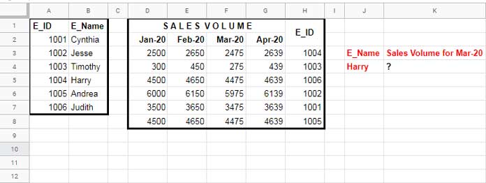
Problem: Get Harry’s sales volume for March
Since Harry’s name is not in the first column of Table 1, we can’t use VLOOKUP directly.
Step 1: Rearrange Table 1 using HSTACK to make name the first column
=VLOOKUP("Harry", HSTACK(B2:B, A2:A), 2, 0)This formula gets Harry’s Employee ID.
Step 2: Rearrange Table 2 so Employee ID comes first
=VLOOKUP(VLOOKUP("Harry", HSTACK(B2:B, A2:A), 2, 0), HSTACK(H3:H, D3:G), 4, 0)Result: Harry’s sales volume in March
Even though March is the 3rd column in the original table, it’s now the 4th column in the reordered table, which is why we use 4 as the column index.
Wrapping Up
That’s everything you need to know about using a nested VLOOKUP in Google Sheets. From looking up values across multiple tables to reordering columns to overcome lookup limitations, nested VLOOKUPs can be very powerful when used correctly.