Assume you have a column with several keywords and want to highlight a bunch of them with a single formula rule. What’s the best option? When you want to highlight using multiple OR in conditional formatting, you can use the REGEXMATCH function in Google Sheets.

Of course, there is the OR logical function. That will work pretty well in conditional formatting.

Using the OR function also, you can include several conditions, but REGEXMATCH is the smartest one.

Other than these two functions, there are options like MATCH, XMATCH, SEARCH, FIND, etc. We will see that also in a later part.

Why the REGEXMATCH function is the better option in multiple OR criteria in conditional formatting rules?

You will get the following advantages when you use the REGEXMATCH in conditional formatting in Google Sheets.

• It’s easy to add multiple conditions.
• The formula will be clean looking.
• A partial match of keywords is possible.
• Case sensitivity.

To make you understand this, I have included enough examples below. So here we go!

The OR Function to Highlight Multiple Keywords in Google Sheets

Syntax: OR(logical_expression1, [logical_expression2, …])

Here I have included only three keywords in my formula. But you can include many more keywords.

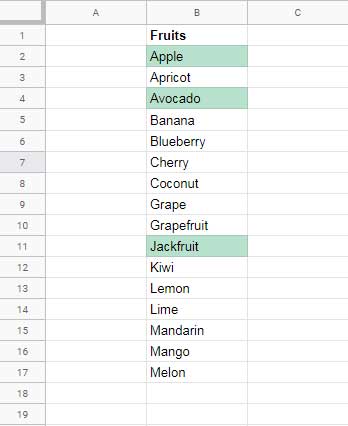
I have used the below OR formula to highlight the keywords “Apple,” “Avocado,” and “Jackfruit” in column B.

=OR(B2="Apple",B2="Avocado",B2="Jackfruit")

Some of you may be new to highlighting, I mean conditional formatting, in Google Sheets. If so, here are the steps to apply the above formula as the custom rule.

Steps:

1. Go to the menu Format > Conditional formatting.
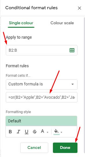
2. We want to highlight B2:B. So enter B2:B in the “Apply to range” in conditional formatting.
3. Then enter my above custom formula under the relevant field. Please see the screenshot below.

It is one of the methods to apply multiple OR in conditional formatting in Google Sheets. Now let’s try the Regex way of highlighting a column with a list of keywords.

REGEXMATCH to Include Multiple OR in Conditional Formatting in Google Sheets

Syntax: REGEXMATCH(text, regular_expression)

All the steps are the same as per the above example, except for the formula.

Here is that REGEXMATCH formula equivalent to the above multiple Logical OR.

=REGEXMATCH(B2,"Apple|Avocado|Jackfruit")

I find this one useful as we can add more conditions easily here. We only need to separate the conditions with the pipe symbol.

This formula has two ‘issues’ though. To test them, I am modifying the sample data and the formula now.

Issue # 1: Partial Match

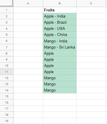
Suppose some of the fruit names contain the country of origin as below.

What happens when we use the below custom rule for the range B2:B?

=REGEXMATCH(B2,"Apple|Mango")

It would highlight all the values as REGEXMATCH partially matches the keywords. It won’t differentiate “Apple” and “Apple – Brazil.”

Then how to highlight the exact match using the REGEXMATCH formula in Google Sheets?

We can use anchors in REGEXMATCH to make it exactly match. Here is an example formula.

=REGEXMATCH(B2,"^Apple$|^Mango$")

This regex formula will only highlight the last seven cells (B8:B14). Please refer to the screenshot above.

Issue # 2: Case Sensitivity

Case sensitivity is the second ‘issue’ you may face when using REGEXMATCH in multiple OR conditional formatting in Google Sheets.

All the above Regex-based rules are case-sensitive. They will treat “Apple” and “APPLE” as two different texts.

How do we solve that?

Specify (?i) to make the content matching case-insensitive.

Example 1: =REGEXMATCH(B2,"(?i)Apple|Mango")

Example 2: =REGEXMATCH(B2,"(?i)^Apple$|^Mango$")

Criteria (Conditions) As a List in a Column in Conditional Formatting

I know it’s impractical to type a long list of keywords in the OR or REGEXMATCH.

It is better to keep the keywords to highlight as a list and refer to that list in the formula.

Using Regex, you can refer to a long list that contains multiple criteria to highlight.

How do we do that?

With the help of the TEXTJOIN function, you can combine the criteria list and place the pipe symbol in between.

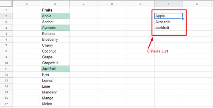
In the following example, the conditions are in the range F2:F4. The column to highlight is column B (B2:B).

Partial (Case Sensitive) Match:

=REGEXMATCH(B2,textjoin("|",true,$F$2:$F$6))

Exact (Case Sensitive) Match:

=REGEXMATCH(B2,"^"&textjoin("$|^",true,$F$2:$F$6)&"$")

Exact (Case Insensitive) Match:

=REGEXMATCH(B2,"(?i)^"&textjoin("$|^",true,$F$2:$F$6)&"$")

The above (OR and REGEXMATCH) are not the only options for multiple OR in conditional formatting in Google Sheets. We can also use functions like MATCH, XMATCH, SEARCH, FIND, etc.

You may also want to try that if you are a Google Sheets enthusiast.

Multiple OR in Conditional Formatting: Alternative Highlight Rules

Remember! The following rules are for the same fruit list in column B, and the “Apply to range” is B2:B.

MATCH and XMATCH Rules

MATCH and XMATCH are two similar functions. They differ feature-wise. We will start with the former function.

Criteria Hardcoded:

=MATCH(B2,TOCOL({"Apple","Avocado","Jackfruit"}),0)

Criteria as a List (Cell Range):

Assume the criteria are available to specify as a list in F2:F. Then specify 1 within TOCOL to remove the blank cells in this criteria range.

=MATCH(B2,TOCOL($F$2:$F,1),0)

What about XMATCH alternative to multiple OR in highlighting?

Syntax: XMATCH(search_key, lookup_range, [match_mode], [search_mode])

Just replace the function name in the formulas above. That’s it. But one thing! As I said above, XMATCH is much more powerful compared to its sibling.

It can also perform wildcard matches. I’m skipping that part since we have Regx for the same above.

SEARCH and FIND Rules

I don’t suggest the following formulas since we have seen much simpler options above.

FIND and SEARCH are two similar functions. The former is case-sensitive, and the latter is not. That’s their difference. Also, both will partially match the criteria in the given range.

If you use SEARCH as an alternative to multiple OR in Google Sheets, try this.

Syntax: SEARCH(search_for, text_to_search, [starting_at])

Criteria Hardcoded:

=ARRAYFORMULA(SUM(IFERROR(SEARCH(TOCOL({"Apple","Avocado","Jackfruit"}),B2))))

Criteria as a List (Cell Range):

=ARRAYFORMULA(SUM(IFERROR(SEARCH(TOCOL($F$2:$F,1),B2))))

In both these, replace SEARCH with FIND for a case-sensitive match.