With the help of the Query function, it’s easy to move each set of rows to columns in Google Sheets. How?

First, let me explain the term ‘each set of rows.’

What I meant to convey is moving each set of ‘n’ rows to columns. Here ‘n’ can be any number of rows.

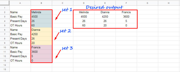
Before coding the formula, see the below image to understand my concept even better.

In this example, column B contains the source data. I have highlighted each set of rows that I want to move to columns with different colors.

Here each set contains a fixed number of (4) rows.

On the right-hand side of the source data, i.e., in the range D2:F5, you can see the moved values.

Here comes a genuine doubt. Can we use the TRANSPOSE function to move each set of rows to columns in Google Sheets?

Nope! That’s not possible. The TRANSPOSE alone can’t do that. I am going to use a Query + TRANSPOSE combo (option # 1) for this.

As a side note, we can also use Vlookup + Transpose combo (option # 2) for this. It’s somewhat complicated-looking compared to the Query + Transpose combo. But better as it expands itself. No user interaction is required.

Let’s come back to the topic.

To flip data, you can use the TRANSPOSE function. But it won’t work with each ‘n’ set of rows. As an example, try the below TRANSPOSE formula.

=transpose(B2:B13)

It would return the entire rows to a single row in several columns.

Two Formulas to Move Each Set of Rows to Columns in Google Sheets

In the following two options, the second one is a dynamic formula. A little complex in nature. But worth trying.

Query Skipping (Option 1)

I am going to use the SKIPPING clause in Query here. We have benefitted from this clause earlier also – How to Move Values in Every Alternate Row to Columns in Google Sheets.

Just enter the below combination formula in cell D2. In this formula, you can see that I have fed the skipping clause with the number 4.

=transpose(query(B2:B,"Select * skipping 4",0))

Note:- Before proceeding, you must format column B to “Plain text” (available in the Format menu). For more details, please see the troubleshooting section below.

Since each set contains four rows, drag the above formula to 3 more rows down. I’ll explain this later. Right now, just understand one thing.

You must drag the formula based on the ‘n’ value in the skipping clause. If you want to skip 10 rows, you should drag the formula down to 9 more rows (total 10 rows).

When each set contains 10 rows, the formula would be as below.

=transpose(query(B2:B,"Select * skipping 10",0))

Vlookup Rows (Option 2) – Recommended ✓

Here is a dynamic formula to move each set of rows to columns in Google Sheets.

In cell D2, insert the following Vlookup formula. It will take care of the rest. You do not require to copy/drag this formula to down or right.

Only make sure that there are no blank cells in the range (B2:B13) to move. If blank, insert 0 or a space character by simply tapping the spacebar.

=ArrayFormula(
     vlookup(
        transpose(sequence(roundup(counta(B2:B)/4),4,row(B2))),
        {row(B2:B),B2:B},
        2,
        0
     )
)

I have used the number 4 two times in the formula. That controls the set of rows to move to columns.

If you want to move three rows each to columns, change both of the 4 to 3.

Can you explain to me how these formulas work? Yes! Here are the formula explanations.

1. Query Skipping Clause – The Combo to Move N Rows to Columns (Explanation)

Syntax:

[skipping n]

n – the number of rows (items) to skip.

See this Query formula that uses the Skipping clause.

=query(B2:B,"Select * skipping 4",0)

Skipping 4 rows, skips four rows and retains the top rows.

Transposing the above Query output would change its orientation.

=transpose(query(B2:B,"Select * skipping 4",0))

When you drag this formula down, the skipping range B2:B becomes B3:B in cell D3, B4:B in cell D4, and B5:B in cell D5.

For example, here is the formula in cell D3.

=transpose(query(B3:B,"Select * skipping 4",0))

See now how the above formula skips/moves each set of rows to columns.

Here instead of cell B2, the skipping starts from cell B3. So the values 4500, 4250, and 3600 move to columns.

The same happens with the copied formulas in cells D4 and D5.

Skipping ‘n’ Rows – Troubleshooting

When you try my formula, you may face a few issues based on your source data. I’ll try to sort out that in this section.

Query Mixed Data Type Issue in Moving ‘n’ Rows to Columns

The above formula has one issue. In order to work the above formula correctly, you must follow either of the below steps.

1. Select the source data (here B2:B) and format it to text (Format > Number > Plain Text). I have followed this tip in my above example.
2. Use the To_Text function as below.

=ArrayFormula(transpose(query(to_text(B2:B),"Select * skipping 4",0)))

See, I have wrapped the source range with the To_Text function.

Since you are using a non-array function (To_text) in an array (range), you must enter the formula as an Array Formula.

That’s why the ArrayFormula in front of the “transpose” above.

This formatting is required because of the ‘unpredictable’ behavior of Query in mixed data type columns like in the range B2:B.

So what about the numbers in the formula output. Can I use that in calculations?

How to Use the Numbers Formatted as Text in Calculations

Since we have formatted the source data to pure text, each set of rows that moved to columns will retain the same formatting. So if you want to perform any calculation that involving numbers, do as follows.

As an example, to SUM D3:D5, use the formula as below.

=ArrayFormula(sum(D3:D5*1))

Please note that the below formula won’t work.

=sum(D3:D5)

Array Formula Occupies Additional Blank Columns

The below image speaks better.

Since we have used the range B2:B, it causes lots of blank rows in the output.

Due to the involvement of the function Transpose in the output, those blank rows flipped to columns.

Due to this, all the columns to the right-hand side of the output have been occupied.

It remains blank, but you are not permitted to enter any values there.

We can solve that using the FILTER function with the formula as below.

Similar: Remove Extra Blank Cells in ArrayFormula Output at the Bottom.

Here is the new formula to be used in cell D2. In this, I have used the Filter around the range to filter out blank rows. Drag down this formula.

=transpose(query(filter(B2:B,len(B2:B)),"Select * skipping 4",0))

2. Vlookup – The Dynamic Formula to Move Each Set of Rows to Columns (Explanation)

The formula will be simple if you know the use of the Sequence function in Google Sheets.

=SEQUENCE(roundup(counta(B2:B)/4),4,row(B2))

Syntax: SEQUENCE(rows, [columns], [start], [step])

rows – roundup(counta(B2:B)/4) – it returns 3.

The Counta count function counts the values in B2:B and divides that result by the number 4 because we want to move each set of four rows to columns.

columns – 4

Output the sequence numbers in four columns.

If we put 1 here, we will only get three numbers in one column. We want to get all the numbers in counta, and that is 12 (3 rows x 4 columns = 12).

Please refer to the range D2:G4 on the image below.

start – 2

The numbering starts from 2.

step – omitted

See what happens when we transpose the same in the range D7:F10.

The above is actually the row numbers of the range B2:B13 arranged in a particular order.

The above-transposed row numbers are the search keys in Vlookup. And the search range is {row(B2:B),B2:B}

The Vlookup searches the row numbers (transposed Sequence output) in the first column of the search range and returns values from the second column.

That’s all.

Follow the above tips and tricks to move each set of rows to columns in Google Sheets. Enjoy!

Related:

• Move Single Column to Multiple Columns Using Hlookup in Google Sheets.
• Split a Column into Multiple N Columns In Google Sheets.