


")


")

")
")
 in Excel & Google Sheets")


We can use the MIN, MINA, and SMALL functions to find minimum values in a range without applying any conditions. Additionally, the SORTN function can sort data and return the smallest value. In this tutorial, let’s explore how to use Min in VLOOKUP in Google Sheets by combining it with these functions to return matching values.
Introduction to VLOOKUP
The VLOOKUP function is one of the most popular lookup functions in Google Sheets. While many users are now switching to XLOOKUP, its successor, VLOOKUP still has its own strengths — especially when it comes to specifying a range instead of separate lookup and result columns, and returning 2D results.
VLOOKUP(search_key, range, index, [is_sorted])When using MIN, MINA, or SMALL in VLOOKUP, we’ll place the output of these functions in the search_key part of the formula. Let’s go through some examples to help you understand this concept better.
1. MIN Function with VLOOKUP
I have sample data where the total budget of a few campaigns is in column A and the campaign names are in column B. See how we can find the minimum budget and return the corresponding campaign name.
=VLOOKUP(MIN(A2:A), A2:B, 2, 0)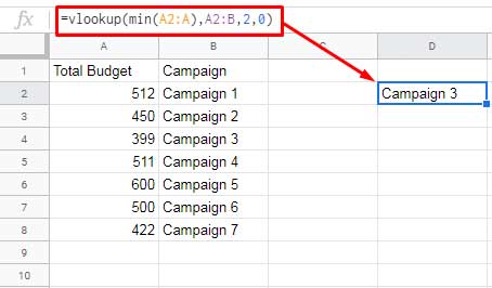
This is a basic example of using Min in VLOOKUP in Google Sheets. The MIN function returns the smallest value in column A, which VLOOKUP then uses as the search_key. Since the minimum value is in the first column of the range, the lookup works perfectly.
When MIN is Not in the First Column
This is a common scenario. For instance, if campaign names are in column A and budgets are in column B, we need to flip the columns so the column with the minimum value (budgets) becomes the first in the range.
You can do this virtually using an array literal:
={B1:B, A1:A}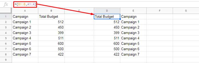
Or, use the HSTACK function:
=VLOOKUP(MIN(B2:B), {B2:B, A2:A}, 2, 0)
=VLOOKUP(MIN(B2:B), HSTACK(B2:B, A2:A), 2, 0)
This is an example of using Min in reverse VLOOKUP.
2. MINA Function in VLOOKUP
To look up the minimum value using VLOOKUP, we may sometimes prefer MINA instead of MIN — especially when the column contains text values.
For example, if the word “Nil” is used in a column to indicate an absence and should be treated as 0, MINA is a better choice because it treats text as 0.
But there’s a catch: MINA will return 0, and VLOOKUP will try to find 0 in the first column of the range. If the value in the cell is “Nil” (a string), the lookup will fail.
How to Handle Text Values Treated as 0
We must convert text values to numbers, replacing them with 0 while retaining other values. The N function can help here, but since it’s not an array function, wrap it with ArrayFormula.
Here’s how:
=ArrayFormula(VLOOKUP(MINA(A2:A), {N(A2:A), B2:B}, 2, 0))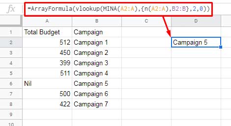
Note: This method isn’t foolproof. If multiple strings exist in the column, the formula will return the first match only.
3. SMALL Function in VLOOKUP
If you want to use VLOOKUP to return the second, third, or any other smallest value in Google Sheets, use the SMALL function instead of MIN.
Here are two examples:
=VLOOKUP(SMALL(A2:A, 2), A2:B, 2, 0)
=VLOOKUP(SMALL(A2:A, 3), A2:B, 2, 0)
These formulas return the values corresponding to the second and third smallest numbers in column A, respectively.
4. SORTN with VLOOKUP
Similar to MIN, you can also use SORTN to return the minimum value before using it as the search key in VLOOKUP.
=VLOOKUP(SORTN(A2:A), A2:B, 2, FALSE)The SORTN function returns the smallest value in the range, and VLOOKUP then finds the corresponding value in column B.
Return the Min Value in Each Group
In this example, the VLOOKUP search key is not the result of MIN, MINA, or SMALL. Instead, we are looking for the minimum value within each group.
Example: VLOOKUP to Return Min Value in Each Group
Suppose we want to find the minimum value of “Campaign 1” in column 3, which is 25. The search key is “Campaign 1”.
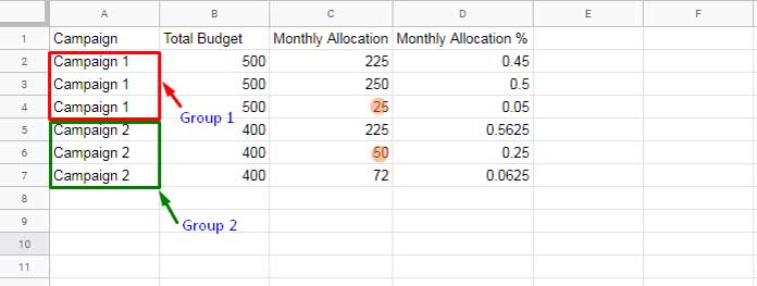
To make this work, sort the data by column 3 in ascending order inside the VLOOKUP:
=VLOOKUP("Campaign 1", SORT(A2:D, 3, TRUE), 3, 0)This formula will return 25 — the minimum value in the group “Campaign 1”.
Return the Min Value of Each Group Dynamically
Use this formula if you want to return the minimum value for multiple groups:
=ArrayFormula(VLOOKUP({"Campaign 1";"Campaign 2"}, SORT(A2:D, 3, TRUE), 3, 0))Or use UNIQUE for a dynamic approach:
=ArrayFormula(IFERROR(VLOOKUP(UNIQUE(A2:A), SORT(A2:D, 3, TRUE), 3, 0)))Resources
👉 Looking for a method to return a value from another column based on the minimum using functions like INDEX-MATCH or FILTER? Check out this guide:
Find Minimum Value and Return Value from Another Column in Google Sheets