
")

")
")


")


")


The most flexible way to find the top N values with criteria in Google Sheets is by combining SORTN and FILTER. The MAX or LARGE functions alone don’t support criteria, and while MAXIFS can return the maximum value based on criteria, it doesn’t return the top N values.
To extract the top N values with criteria, we use FILTER to apply the condition and SORTN to select the highest values from the filtered data.
SORTN also provides four tie-handling modes, allowing you to control how duplicates are treated when multiple values share the same rank.
Below, we’ll explore four different formulas, so you can choose the one that fits your needs.
Sample Data
The sample dataset contains total sales for seven products across different months. Suppose we need to find the top three sales values for January.
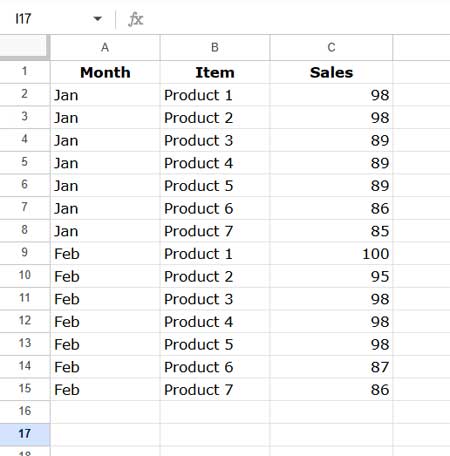
The criteria will be “Jan” in Column A.
Generic Formula
Use the following formula structure to find the top N values with criteria:
=SORTN(FILTER(data, criteria), n, ties_mode, index, FALSE)Where:
data: The dataset from which to extract the top N values.criteria: The condition that filters relevant data.n: The number of top values to return.ties_mode: Defines how to handle duplicate values.index: The column containing the numerical values to rank.
Now, let’s explore different ways to find top N values with criteria in Google Sheets using various ties_mode options.
1. Find Top N Values with Criteria – Exact Top N Values
To find the top three sales values for January, use this formula:
=SORTN(FILTER(A2:C, A2:A="Jan"), 3, 0, 3, FALSE)How It Works:
FILTER(A2:C, A2:A="Jan"): Filters the dataset for January.SORTN(..., 3, 0, 3, FALSE): Sorts by Column 3 (Sales) in descending order and returns the top 3 values.
Result:
| Month | Item | Sales |
| Jan | Product 1 | 98 |
| Jan | Product 2 | 98 |
| Jan | Product 3 | 89 |
👉 This method only returns exactly three values, even if there are duplicates.
2. Find Top N Values + Duplicates of the Nth Value
This formula returns the top N values plus any additional duplicates of the Nth value.
=SORTN(FILTER(A2:C, A2:A="Jan"), 3, 1, 3, FALSE)Result:
| Month | Item | Sales |
| Jan | Product 1 | 98 |
| Jan | Product 2 | 98 |
| Jan | Product 3 | 89 |
| Jan | Product 4 | 89 |
| Jan | Product 5 | 89 |
👉 Since 89 is the third-highest value, all rows with 89 are also included.
3. Find Top N Unique Values
To return only the top 3 unique sales values, use:
=SORTN(FILTER(A2:C, A2:A="Jan"), 3, 2, 3, FALSE)Result:
| Month | Item | Sales |
| Jan | Product 1 | 98 |
| Jan | Product 3 | 89 |
| Jan | Product 6 | 86 |
👉 This formula ignores duplicates and returns only unique values.
4. Find Top N Unique Values + All Their Duplicates
If you need top N unique values plus all their duplicates, try:
=SORTN(FILTER(A2:C, A2:A="Jan"), 3, 3, 3, FALSE)Result:
| Month | Item | Sales |
| Jan | Product 1 | 98 |
| Jan | Product 2 | 98 |
| Jan | Product 3 | 89 |
| Jan | Product 4 | 89 |
| Jan | Product 5 | 89 |
| Jan | Product 6 | 86 |
👉 This formula returns top unique values along with all duplicate instances.
Adding Multiple Criteria
To apply multiple criteria, modify the FILTER function accordingly.
For example, to exclude “Product 1” from the evaluation:
=FILTER(A2:C, A2:A="Jan", B2:B<>"Product 1")If you want to exclude both “Product 1” and “Product 5”:
=FILTER(A2:C, A2:A="Jan", (B2:B<>"Product 1")*(B2:B<>"Product 5"))Conclusion
Finding the top N values with criteria in Google Sheets is simple and flexible with FILTER and SORTN. With four different tie-handling options, you can customize the results to match your needs—whether you want exact values, unique values, or duplicates included.
By understanding these formulas, you can efficiently extract the top N values for any dataset without manual filtering or sorting!
SHOULD BE NICE IF YOU SHARE A GOOGLE SHEET WITH THIS EXERCISE.
THANKS.