If you have a dataset with dates spread across columns, you might want to quickly pull the latest date per row—for example, the last activity date for each employee or student.

The MAX function works well for a single row, but if you want to apply it across all rows without dragging down the formula, you’ll need an array formula.

In this tutorial, we’ll explore:

• How to get the max date in each row with a simple drag-down formula.
• The modern BYROW + LAMBDA solution that spills results automatically.
• An old-school DMAX workaround (useful for learning).

Sample Data

Here’s a small dataset of employees and their activity dates:

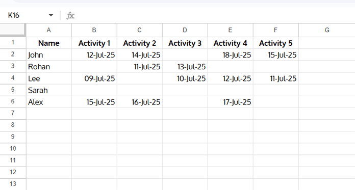
We want to return the latest (max) activity date for each employee in a new column.

Non-Array Formula (Drag-Down)

The simplest approach is to use MAX row by row:

=MAX(B2:F2)

Placed in G2 and dragged down, this gives the latest date in each row.

But there’s a catch:

If the row is empty, it may return 0 or show as 30-Dec-1899 (the zero date in Sheets). To fix this, here are three better versions.

• Returns a properly formatted date or blank.

=TO_DATE(IFERROR(1/MAX(B2:F2)^-1))

• Retains the dataset’s date formatting, my preferred method.

=IF(MAX(B2:F2), MAX(B2:F2),)

• Uses FILTER to ignore blanks.

=TO_DATE(IFNA(MAX(FILTER(B2:F2, B2:F2))))

These all work—but they need to be copied down manually.

Array Formula with BYROW + LAMBDA to Get Max Date in Each Row

With BYROW and LAMBDA, you can create a fully dynamic formula that updates automatically for all rows.

=BYROW(B2:F, LAMBDA(row, IF(MAX(row), MAX(row),)))

How it works:

• BYROW(B2:F, …) → processes each row in the range individually.
• MAX(row) → finds the latest date in that row.
• IF(MAX(row), MAX(row), ) → ensures empty rows return blank instead of 0.

✅ Advantages:

• Automatically handles new rows.
• Much cleaner sheet (only one formula).
• Future-proof and scalable.

DMAX Workaround to Get Max Date in Each Row

Before BYROW and LAMBDA were introduced, power users relied on the DMAX trick.

Here’s the array formula version:

=ArrayFormula(
   TO_DATE(
      IFERROR(1/DMAX(
         VSTACK(, TRANSPOSE(B2:F)), 
         SEQUENCE(ROWS(B2:B)), 
         VSTACK(IF(,,), IF(,,))
      )^-1)
   )
)

Explanation:

• TRANSPOSE(B2:F) → flips rows into columns since DMAX only works column-wise.
• VSTACK("", …) → adds a fake header row (DMAX requires one).
• SEQUENCE(ROWS(B2:B)) → generates column references dynamically.
• 1/x^-1 → forces an error on empty rows, avoiding the zero date.
• IFERROR + TO_DATE → ensures clean date formatting.

While clever, this method is now more of a formula curiosity. For everyday work, stick with BYROW or the simple drag-down solution.

Conclusion

To get the max date in each row in Google Sheets:

• Use MAX(B2:F2) with an IF or IFERROR wrapper if you don’t mind dragging down.
• Use the BYROW + LAMBDA formula for a modern, dynamic, one-formula solution.
• The DMAX workaround is good to know but outdated for most use cases.

If your goal is a clean, scalable sheet, the BYROW + LAMBDA approach is the best option today.

Related Resources

• Highlight Largest 3 Values in Each Row in Google Sheets (+ Ties)
• How to Find Max Value in Each Row in Google Sheets
• Find Max N Values in a Row and Return Headers in Google Sheets
• How to Highlight Max Value in a Row in Google Sheets
• Find Min or Max in a Google Sheets Matrix and Return Row Data
• Return First and Second Highest Values in Each Row in Google Sheets