


")


")

")
")
 in Excel & Google Sheets")


You can use the FILTER function to lookup a header and filter all non-blank values in that column in Google Sheets. Additionally, you can include the corresponding values from the first column of the table.
Generic Formulas
=LET(ftr, FILTER(data, row=G2), FILTER(ftr, ftr<>""))- Replace data with the range to filter (excluding the header row).
- Replace row with the first-row reference of the data.
- Replace G2 with the column header to lookup.
If you want to include the first column along with the filtered lookup column, use this formula:
=LET(ftr, FILTER(data, (row=G2)+(row=G3)), FILTER(ftr, CHOOSECOLS(ftr, 2)<>""))Additionally, specify the first column header label in G3.
Let’s go through two examples to understand how to lookup a header, filter non-blanks in the found column, and optionally include the first column.
Example 1: Lookup Header and Filter Non-Blanks in the Lookup Column
Imagine you have a dataset where each column represents sales data for different regions (e.g., “North,” “South,” “East,” “West”), and the rows contain monthly sales figures. The first column contains month names. Some cells may be blank if there were no sales in a given month.
The goal is to dynamically select a region (column) by specifying the header (e.g., “East”). Once the column is identified, we extract only the non-blank sales values from that column for further analysis.
Sample Data (A1:E)
| Month | North | South | East | West |
| Jan | 350 | 150 | 50 | -150 |
| Feb | 250 | 100 | 450 | |
| Mar | 300 | 200 | 350 | |
| Apr | 330 | 220 | 120 | 400 |
Enter the region you want to lookup in G2, for example, “East”.
Enter the following formula in H2 to filter the column corresponding to the lookup value while removing blanks:
=LET(ftr, FILTER(A2:E5, A1:E1=G2), FILTER(ftr, ftr<>""))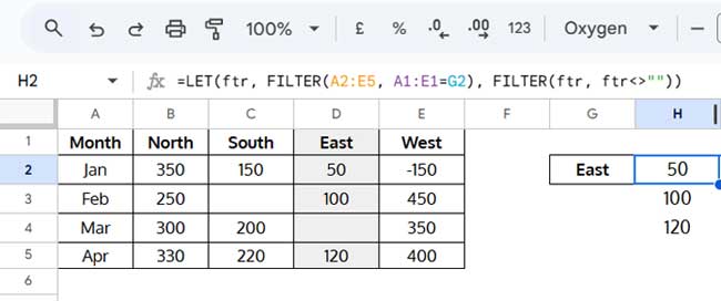
Formula Breakdown
FILTER(A2:E5, A1:E1=G2)– Filters the range A2:E5, selecting the column where the header in A1:E1 matches G2.- We use LET to name this result ftr.
FILTER(ftr, ftr<>"")– Further filters ftr to remove blank cells.
Example 2: Lookup Header and Filter Non-Blanks + First Column
This time, the goal is to filter the selected region’s column while also including the first column.
Enter the region “East” in G2 and the first column header, i.e., “Month”, in G3.
Then, use this formula:
=LET(ftr, FILTER(A2:E5, (A1:E1=G2)+(A1:E1=G3)), FILTER(ftr, CHOOSECOLS(ftr, 2)<>""))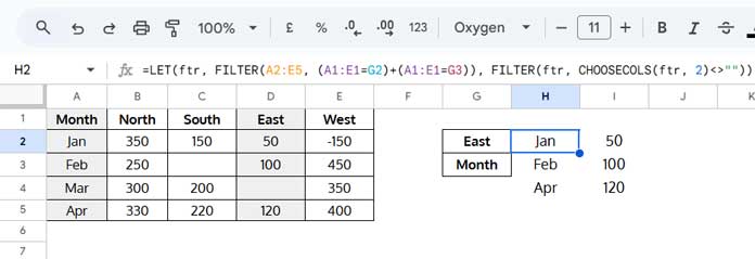
There is a specific benefit to including the first column. It helps identify the specific months with sales along with the sales figures.
Formula Explanation
FILTER(A2:E5, (A1:E1=G2)+(A1:E1=G3))– Filters A2:E5, selecting columns where the header matches G2 (East) or G3 (Month).- We use LET to name this result ftr.
FILTER(ftr, CHOOSECOLS(ftr, 2)<>"")– Ensures that only rows where the second column (East) is non-blank are returned.
Additional Tip
In both formulas, you can replace <>"" with >0 to filter out empty and zero-value rows:
=LET(ftr, FILTER(A2:E5, A1:E1=G2), FILTER(ftr, ftr>0))
=LET(ftr, FILTER(A2:E5, (A1:E1=G2)+(A1:E1=G3)), FILTER(ftr, CHOOSECOLS(ftr, 2)>0))