


")


")

")
")
 in Excel & Google Sheets")


The LIST_ALL_DATES custom named function in Google Sheets lets you quickly generate date ranges by listing every date between a start date and an end date.
Unlike regular formulas, this function can also assign values from other cells or ranges to each expanded date, making it especially useful for project timelines, schedules, and task tracking.
Below are examples to help you understand how this named function works. You can download the example sheet and try it out in your own Google Sheets.
👉 In all examples, only the cyan-highlighted cells contain formulas.
Examples
1. List all dates between a single start date and end date
Formula in C3:
=LIST_ALL_DATES(A3, B3, "")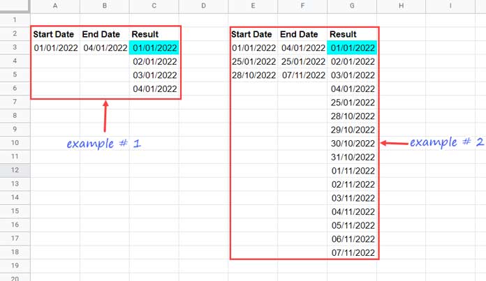
2. List all dates between multiple start and end dates
Formula in G3 (using ArrayFormula):
=ArrayFormula(LIST_ALL_DATES(E3:E, F3:F, IFERROR(E3:E/0)))Here, we don’t want to use the last argument. Instead, we create a virtual blank column with IFERROR(E3:E/0). Alternatively, you can reference a real blank column, e.g.:
=LIST_ALL_DATES(E3:E, F3:F, J3:J)(ensure J3:J is empty)
3. Expand dates and assign a single value
Formula in D3:
=LIST_ALL_DATES(A3, B3, C3)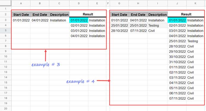
4. Expand multiple date ranges and assign corresponding values
Formula in J3:
=LIST_ALL_DATES(G3:G, H3:H, I3:I)In Example 4, the additional values come from a single column, but the function also supports multiple ranges.
Syntax and Arguments of LIST_ALL_DATES
LIST_ALL_DATES(start_date_range, end_date_range, additional_range)Arguments:
- start_date_range → A cell or single-column range containing start date(s).
Example:A2orA2:A - end_date_range → A cell or single-column range containing end date(s).
Example:B2orB2:B - additional_range → A cell or range containing values to assign to the generated dates.
Example:C2orC2:C
👉 You can include multiple columns in this argument by combining them with the ~ delimiter, e.g.:
=ArrayFormula(LIST_ALL_DATES(A2:A, B2:B, C2:C&"~"&D2:D))If you don’t want to use the last argument, specify an empty cell or a blank range.
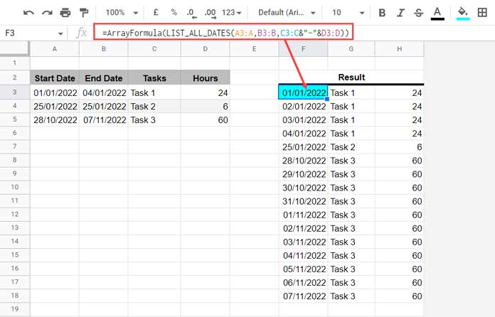
How to Use More Than One Additional Range
For example, suppose you have:
- Start dates →
A3:A - End dates →
B3:B - Tasks →
C3:C - Man-hours →
D3:D
You can combine tasks and man-hours into a single column using the ~ delimiter:
=ArrayFormula(LIST_ALL_DATES(A3:A, B3:B, C3:C&"~"&D3:D))This will list every date in the ranges along with the task and man-hours for each.
Important Notes and Limitations
- The function outputs date values. To display them correctly, select the results and apply Format > Number > Date.
- You can copy the function from the example sheet below.
- For details on how to import and use named functions in Google Sheets, see: Named Functions in Google Sheets.
- ⚠️ Performance Warning: Since this function is built with LAMBDA functions, it can be resource-intensive. On larger datasets, it may slow down your spreadsheet or stop working altogether.
Related Tutorial
If you prefer not to use a named function, check out:
👉 Expand Dates and Assign Values in Google Sheets (Array Formula)