As a business owner, you may have your own reasons to find the last working day of a year, such as strategic planning or holiday preparation. You can do this easily using a formula in Google Sheets.

What you need to do is provide the year. The formula will return the last working day of that year. Additionally, by using the YEAR function with TODAY, you can find the last business day of the current year, the previous year, or the next year.

You can use the WORKDAY.INTL function for this purpose. Here’s the formula:

=WORKDAY.INTL(DATE(year, 12, 31)+1,-1, [weekend], [holiday_range])

In this formula:

• Replace year with the year for which you want to find the last business day.
• Replace holiday_range with the range of cells containing specific holidays you want to exclude.
• Specify the weekend parameter if your weekends are not Saturday and Sunday.

Determining Weekends (String Method)

There are two methods to specify weekends in the function: Number and String.

The string method is the easiest way to specify weekends, so we’ll use it here.

In this method, you specify 7 digits (0s and 1s) representing Monday to Sunday, where 0 indicates a working day and 1 indicates a weekend. For example:

• For Saturday/Sunday weekends, use “0000011”.
• For Friday/Saturday weekends, use “0000110”.

Examples: Finding the Last Business Day of a Year

Example 1: Last Working Day of a Given Year

Assume cell B3 contains the year 2024. Enter the following formula in cell C3 to get the last working day of that year:

=WORKDAY.INTL(DATE(B3, 12, 31)+1, -1)

This formula considers Saturday and Sunday as weekends and excludes no specific holidays.

If you have holidays to exclude, enter those dates in column A (e.g., A3:A) and use this formula:

=WORKDAY.INTL(DATE(B3, 12, 31)+1, -1, "0000011", A3:A)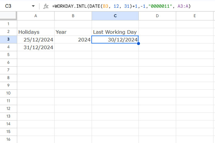

To specify Friday/Saturday as the weekend and exclude holidays from A3:A, use:

=WORKDAY.INTL(DATE(B3, 12, 31)+1, -1, "0000110", A3:A)

How This Formula Works

1. Generating the Last Date of the Year:
   The DATE function generates the last date of the year (e.g., 31/12/2024 for 2024): DATE(B3, 12, 31)
2. Advancing to the Next Year:
   Adding 1 to this date gives the first day of the following year: DATE(B3, 12, 31)+1
3. Counting Backward with WORKDAY.INTL:
   The WORKDAY.INTL function counts backward from this date because of the negative number (-1), returning the last working day of the given year.

Syntax:

WORKDAY.INTL(start_date, num_days, [weekend], [holidays])

Example 2: Finding the Last Working Day of the Current, Previous, or Next Year

To find the last working day for the current, previous, or next year, replace B3 in the formula with one of the following:

• Current Year: Replace B3 with YEAR(TODAY()).
• Previous Year: Replace B3 with YEAR(TODAY())-1.
• Next Year: Replace B3 with YEAR(TODAY())+1.

Related Resources

• Finding the First and Last Workdays of a Month in Google Sheets
• Get the Last Saturday of Any Given Month and Year in Google Sheets
• Finding the Last 7 Working Days in Google Sheets (Array Formula)
• Return All Working Dates Between Two Dates in Google Sheets
• How to Find the Last Business Day of a Month in Excel
• Find the Number of Working and Non-Working Days in Google Sheets
• How to Highlight the Next N Working Days in Google Sheets