


")


")

")
")
 in Excel & Google Sheets")


It’s common to have several empty rows at the bottom of a Google Sheet, especially when you’re reserving space for future data entry. In such cases, how do you get the last row with any data in Google Sheets, particularly when working across multiple columns?
If you’re working with a single column, the task is fairly simple using LOOKUP-based functions.
Get the Last Row in a Single Column
For example, to get the last row in column A, you can use:
=ARRAYFORMULA(XLOOKUP("?*", A:A & "", A:A, , 2, -1))However, this approach doesn’t work when you want to get the last row with any data in Google Sheets across multiple columns—since the last row could have data in just one column, several columns, or all of them.
To solve this, here are two robust methods that work across a 2D range: one using the LAMBDA helper function and another using LOOKUP and SORT logic.
Sample Data
Consider the data in range A1:C:
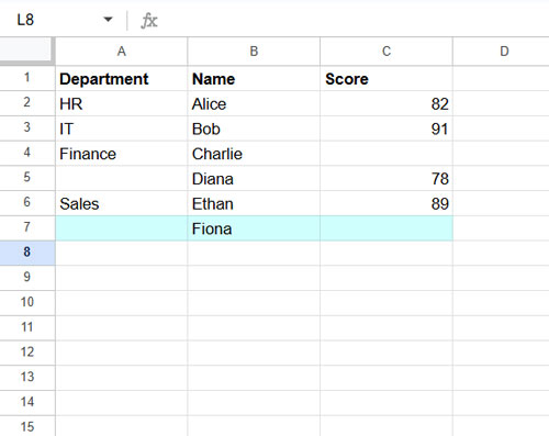
In this case, row 7 is the last row that contains any data—Fiona’s name appears in column B.
Now, how can you retrieve that row from the full range A1:C, without hardcoding A1:C7?
Method 1: Get the Last Row with Any Data – LAMBDA Approach
=CHOOSEROWS(
   A1:C,
   MAX(
      BYROW(A1:C, LAMBDA(val, IF(COUNTA(val), ROW(val))))
   )
)
This formula dynamically returns the last row with any data in a 2D range.
How it works:
BYROW()scans each row and processes it individually.COUNTA(val)counts non-empty cells.IF(..., ROW(val))returns the row number for rows with any data.MAX()gets the highest row number with data.CHOOSEROWS()returns that row from the original range.
Simple and elegant!
To learn more about BYROW, check out: How to Use the BYROW Function in Google Sheets.
Method 2: Get the Last Row with Any Data – Sort & Lookup Approach
While the LAMBDA approach is compact, it might not perform well on very large datasets. In such cases, use this alternative:
=ARRAYFORMULA(
  LET(
    range, TRANSPOSE(A1:C),
    bt, NOT(ISBLANK(range)),
    errv, IF(bt, bt, NA()),
    rseq, SEQUENCE(COLUMNS(errv), 1, -1, -1),
    swap, CHOOSECOLS(errv, rseq),
    row_, SORTN(swap),
    id, -XMATCH(TRUE, row_),
    CHOOSEROWS(A1:C, id)
  )
)
Understanding the Logic
Let’s break down the formula step-by-step using a smaller example like A1:C10:
1. TRANSPOSE(A1:C10)
Rotates the data so rows become columns.
| Department | HR | IT | Finance | Sales | |||||
| Name | Alice | Bob | Charlie | Diana | Ethan | Fiona | |||
| Score | 82 | 91 | 78 | 89 |
2. NOT(ISBLANK(range))
Produces a Boolean array where TRUE marks a cell with data and FALSE marks an empty cell.
| TRUE | TRUE | TRUE | TRUE | FALSE | TRUE | FALSE | FALSE | FALSE | FALSE |
| TRUE | TRUE | TRUE | TRUE | TRUE | TRUE | TRUE | FALSE | FALSE | FALSE |
| TRUE | TRUE | TRUE | FALSE | TRUE | TRUE | FALSE | FALSE | FALSE | FALSE |
3. IF(bt, bt, NA())
Replaces all FALSE values (i.e., blank cells) with #N/A. This helps prevent empty rows from being considered in the next steps.
| TRUE | TRUE | TRUE | TRUE | #N/A | TRUE | #N/A | #N/A | #N/A | #N/A |
| TRUE | TRUE | TRUE | TRUE | TRUE | TRUE | TRUE | #N/A | #N/A | #N/A |
| TRUE | TRUE | TRUE | #N/A | TRUE | TRUE | #N/A | #N/A | #N/A | #N/A |
4. SEQUENCE(...) + CHOOSECOLS(...)
Reverses the column order, effectively flipping the data from right to left. This positions the bottom-most rows of the original range toward the beginning of the array.
| #N/A | #N/A | #N/A | #N/A | TRUE | #N/A | TRUE | TRUE | TRUE | TRUE |
| #N/A | #N/A | #N/A | TRUE | TRUE | TRUE | TRUE | TRUE | TRUE | TRUE |
| #N/A | #N/A | #N/A | #N/A | TRUE | TRUE | #N/A | TRUE | TRUE | TRUE |
5. SORTN(...)
Returns the first row (from the flipped data) that contains at least one TRUE value. This corresponds to the last row with any data in the original orientation.
| #N/A | #N/A | #N/A | TRUE | TRUE | TRUE | TRUE | TRUE | TRUE | TRUE |
6. XMATCH(TRUE, row_)
Identifies the position of the first TRUE in that sorted row. Since the data was reversed, this value tells us how far from the bottom the last row with data is. We negate the result using -XMATCH(...) so it can be used with CHOOSEROWS to return the row from the bottom.
-4
7. CHOOSEROWS(A1:C, id)
Uses the negative index to retrieve the correct row from the bottom of the original range.
This technique is particularly helpful for large or irregular datasets where the LAMBDA approach may slow down. It demonstrates a clever use of transposing, logical masking, and reverse indexing to get the last row with any data in Google Sheets.
Conclusion
You now have two powerful methods to get the last row with any data across multiple columns in Google Sheets:
- LAMBDA + BYROW – best for smaller, more manageable datasets.
- Sort + Lookup Logic – better for larger sheets with potential LAMBDA limitations.
Both approaches allow you to dynamically reference only the relevant portion of your dataset without manually trimming the range.
Related Resources
- Get the Last Column from a Data Range in Google Sheets
- Get the First or Last Row/Column in a New Google Sheets Table
- Pull the Last Row from Multiple Sheets into One in Google Sheets
- Formula to Conditionally Filter Last N Rows in Google Sheets
- 4 Formulas to Last Row Lookup and Array Result in Google Sheets
- Get the First and Last Row Numbers of Items in Google Sheets
- Dynamically Remove Last Empty Rows and Columns in Sheets
- Find the Address of the Last Used Cell in Google Sheets