


")


")

")
")
 in Excel & Google Sheets")


When the lookup key appears more than once, the LOOKUP function returns the result from the last matched row—but it can’t return multiple column outputs. So we can’t rely on it for last row lookup and array result in Google Sheets.
Another limitation: it requires the range to be sorted. That’s not a deal-breaker, though—we can virtually sort the range using SORT.
In this tutorial, I’ll show you 6 different formulas to replace LOOKUP and return array results from the last matching row in Google Sheets. But first, let’s clear a few common doubts.
Understand the Scenario
Here are the two syntax formats for the LOOKUP function:
Syntax 1:
LOOKUP(search_key, search_range, result_range)Syntax 2:
LOOKUP(search_key, search_result_array)Sample Data:
| Item | Ordered | Received |
|---|---|---|
| apple | 100 | 50 |
| apple | 100 | 50 |
| apple | 100 | 75 |
| banana | 500 | 505 |
| mango | 150 | 100 |
| mango | 100 | 110 |
| orange | 100 | 100 |
| orange | 150 | – |
| peer | 100 | 100 |
Sample formulas:
=LOOKUP("apple", A2:C)
=LOOKUP("apple", A2:A, C2:C)
Both formulas search for “apple” in A2:A and return the last received quantity from column C.
But what if you want to return both Ordered and Received quantities?
You can try:
=HSTACK(
   LOOKUP("apple", A2:A, B2:B),
   LOOKUP("apple", A2:A, C2:C)
)
But that gets messy, especially if you want a last row lookup and array result across multiple columns.
Last Row Lookup and Array Result in Google Sheets – 6 Formula Options
The following solutions don’t require the list to be sorted, unlike LOOKUP.
Formula 1: INDEX + FILTER
The search key is the fruit name in cell E2 (e.g., "mango"). We want to get the last Ordered and Received values, found in row #7.
=INDEX(
   FILTER(B2:C, A2:A=E2),
   COUNTIF(A2:A, E2)
)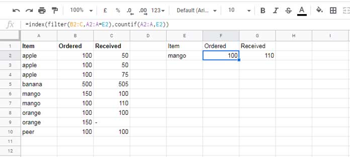
Explanation:
1. FILTER(B2:C, A2:A=E2) gets all rows for “mango”:
| 150 | 100 |
| 100 | 110 |
2. COUNTIF(A2:A, E2) returns the number of matches (2).
3. INDEX(..., 2) returns the last row from the filtered result.
This is a reliable approach for last row lookup and array result in Google Sheets.
Formula 2: XLOOKUP
XLOOKUP supports reverse search and array results. It’s modern and concise:
=XLOOKUP(E2, A2:A, B2:C, , 0, -1)Explanation:
- Searches for E2 from bottom to top (
-1). - Returns matching values from B2:C.
👍 This is my recommended method for last row lookup with array results.
Formula 3: VLOOKUP + FILTER
=ARRAYFORMULA(
   VLOOKUP(
      E2,
      FILTER(A2:C, A2:A=E2),
      {2, 3},
      TRUE
   )
)
Explanation:
1. FILTER(A2:C, A2:A=E2) isolates matching rows.
| mango | 150 | 100 |
| mango | 100 | 110 |
2. VLOOKUP(..., {2,3}, TRUE) looks up and returns columns B and C.
3. Setting is_sorted to TRUE ensures it fetches the last match.
✅ Works well when you need a fast solution with VLOOKUP.
Formula 4: SORTN + FILTER
=SORTN(
   FILTER(B2:C, A2:A=E2),
   1,
   0,
   SEQUENCE(COUNTIF(A2:A, E2), 1),
   FALSE
)
Explanation:
FILTER(B2:C, A2:A=E2)filters the rows by item.SEQUENCE(COUNTIF(...))generates a helper index.SORTN(..., 1, 0, ..., FALSE)returns the last row.
Another neat way to perform a last row lookup and return array result.
Formula 5: CHOOSEROWS + FILTER
=CHOOSEROWS(
   FILTER(B2:C, A2:A=E2), -1
)
Explanation:
FILTER(B2:C, A2:A=E2)pulls all matching rows.CHOOSEROWS(..., -1)gets the last row from the filtered result.
✅ Simple, clean, and perfect for last row lookup with array output.
Formula 6: QUERY Formula
=QUERY(A2:C, "Select B, C where A='"&E2&"' offset "&COUNTIF(A2:A, E2)-1)Explanation:
- Filters rows matching the value in E2.
- Uses
OFFSETto skip to the last row.
Powerful and dynamic way to get the last row lookup and array result in Google Sheets using QUERY.