When you join double quotes with text (at the beginning, end, or both), Google Sheets interprets everything within the quotes as plain text. The quotes themselves are ignored.

="Hello, world!" – This formula will return the string “Hello, world!”.

If you don’t use any quotes around text in a formula, Google Sheets might interpret it as a named range (a custom cell range you’ve defined) or a structured table reference.

For example, the word total in the formula ={total} may be treated as a named range or a table name because there are no double quotation marks around it.

If there is no named range or table name, the formula returns an “Unknown range name: ‘total'” error. On the other hand, total in ={"total"} is treated as text.

How do you concatenate double quotation marks with plain text using a formula in Google Sheets?

Formulas to Join Double Quotes with Text in Google Sheets

You can join double quotes with text or any value in a cell reference in two ways: by concatenating CHAR(34) which represents double quotes or by directly adding double quotes.

Let’s assume cell A1 contains the value to which you want to add double quotes on both sides. You can use either of the below formulas:

=CHAR(34)&A1&CHAR(34)
=""""&A1&""""

You can also use the CONCATENATE function instead of using the ampersand to join the double quotes with the text as follows:

=CONCATENATE(CHAR(34), A1, CHAR(34))
=CONCATENATE("""", A1, """")

This adheres to the syntax CONCATENATE(string1, [string2, …]), where string1, string2, and string3 are CHAR(34), A1, and CHAR(34), respectively.

Concatenating Double Quotes with Multiple Texts

When you want to concatenate double quotation marks with multiple texts and add a comma delimiter in between, you can follow the approach below.

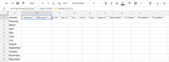
Enter the text in a column, for example, month names in A1:A12.

Then use the following formula in cell B1:

=ArrayFormula(JOIN(",", CHAR(34)&A1:A12&CHAR(34)))

Formula Breakdown:

• CHAR(34)&A1:A12&CHAR(34) – The ampersand joins the double quotes (represented by CHAR(34)) around each string.
• JOIN(",", …) – The JOIN function inserts the comma delimiter to separate each text.

Since it uses an array reference, the formula enters as an array formula.

What’s the Real-Life Use of It?

Let’s consider the output of the above formula in cell B1. To convert the formula result to a static text string, follow these steps:

1. Right-click on cell B1 and click Copy in the context menu.
2. Right-click on cell B1 again and click Paste Special > Values only.

This will convert the formula result in cell B1 to the following text string: "January","February","March","April","May","June","July","August","September","October","November","December"

To convert this string to an array, place curly braces around it and add an equal sign at the beginning, as follows:

={"January","February","March","April","May","June","July","August","September","October","November","December"}

This will return the month names in cells B1:M1. If you want the values in cells B1:B12, replace the comma delimiter in the JOIN formula with a semicolon delimiter.

You can use the above array to sort the month names in a column in chronological order.

Resources

• How to Remove Extra Delimiter in Google Sheets
• How to Concatenate a Number without Losing Its Format in Google Sheets
• How to Properly Concatenate Start Time with End Time in Google Sheets
• Concatenate Header Names with the Values of the Cells Below Them in Google Sheets
• Combine Text and Date in a Google Sheets