")
")


")


")

")
")
 in Excel & Google Sheets")


Explore how to use the ISBETWEEN with FILTER function in Google Sheets, plus when ISBETWEEN doesn’t apply.
Before the ISBETWEEN function, we had to rely on operators such as >, >=, <, or <= to filter data that falls within two values or two dates.
Now, we can replace those operators with the ISBETWEEN function inside the FILTER formula in Google Sheets. This makes formulas much easier to read, and you won’t get confused when you see them in a shared sheet.
ISBETWEEN with FILTER Function Examples
The FILTER function has two arguments: range and condition. We will use the ISBETWEEN with FILTER function as the condition/criteria.
In practice, you can apply conditions in two ways:
- Using two values as the criteria.
- Using two arrays as the criteria.
You can find both explained in Examples 1 and 2 below.
Example 1: Two Values as the Criteria
In the sample data in B3:D, I want to filter the Current Cost wherever the Purchase Date falls between the two dates provided in cells G3 and H3. I also want to consider one more condition: Stock.
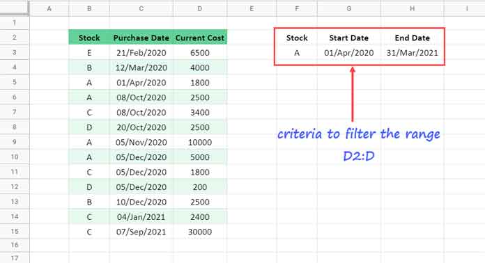
ISBETWEEN with FILTER Function – Example 1
Let’s ignore the Stock criteria for the time being. Here’s the formula:
=FILTER(D3:D, ISBETWEEN(C3:C, G3, H3))This formula filters the Current Cost if the Purchase Date falls between 01-Apr-2020 and 31-Mar-2021 (both dates inclusive).
To filter only a specific Stock, for example A, use:
=FILTER(D3:D, ISBETWEEN(C3:C, G3, H3), B3:B=F3)What if you want to add one more stock?
ISBETWEEN with FILTER Function – Example 2
In that case, you can use OR logic within FILTER, like this (Regex is another option too):
=FILTER(D3:D, ISBETWEEN(C3:C, G3, H3), (B3:B=F3)+(B3:B=F4))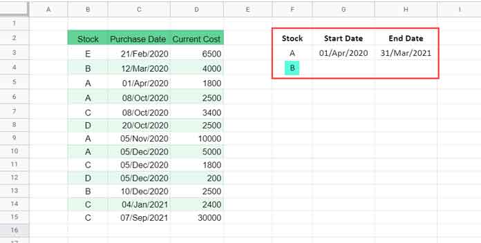
Related: REGEXMATCH in FILTER Criteria in Google Sheets [Examples]
Notes on Using ISBETWEEN with FILTER
- Always try these formulas in a blank column, as they may return multiple rows (array results). Otherwise, you may see a
#REF!error. - By default, both dates in ISBETWEEN are inclusive. To make them exclusive, use:
ISBETWEEN(C3:C, G3, H3, FALSE, FALSE)Example 2: Arrays as the Criteria When Using ISBETWEEN with FILTER
In all the examples above, the criteria were two fixed dates. But sometimes, the criteria can come from two different columns in your dataset.
In other words: you may want to filter values when one column (array) falls between two other arrays.
Here’s a sample scenario:
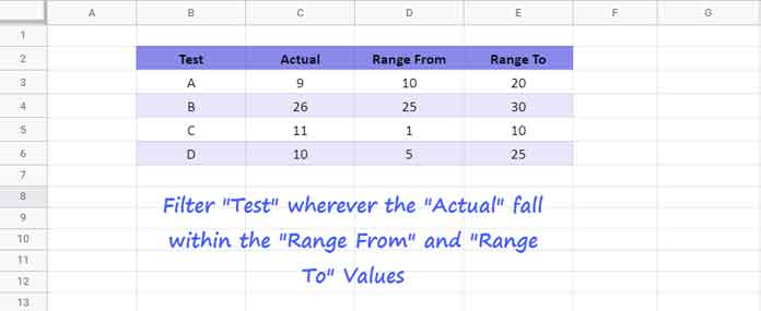
Here, we can filter Test wherever Actual falls within Range From and Range To:
=FILTER(B3:B, ISBETWEEN(C3:C, D3:D, E3:E))The output will be tests B and D.
This is useful when you want to check whether your test results fall within specified ranges and filter the values that do (or don’t).
For the “not falls” case, use:
=FILTER(B3:B, NOT(ISBETWEEN(C3:C, D3:D, E3:E)))👉 I’ve explained this same use case in more detail in my tutorial Find Whether Test Results Fall within Their Limit in Google Sheets, which focuses specifically on test results against their defined ranges.
👉 You can also check my tutorial Visually Track Where Your Data Falls Within Limits (Google Sheets), where I approached the same problem visually using a Sparkline bar with colored ranges and a vertical marker.
Note: When ISBETWEEN Doesn’t Apply
In some scenarios, you may need to check whether a single value falls within multiple row-based ranges (for example, employee work shifts with “Start” and “End” times). Here, ISBETWEEN can’t be used directly because it only works with fixed values or arrays.
Instead, you can use comparison operators within FILTER. For example, to check whether 10:00 falls within each employee’s shift:
=FILTER(A2:A, (B2:B<=TIME(10,0,0)) * (C2:C>=TIME(10,0,0)))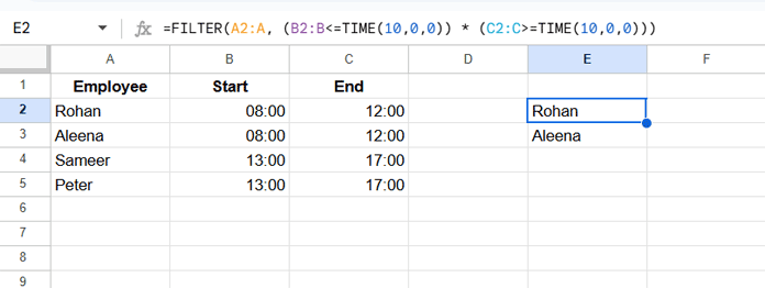
This formula returns the employees who are available at 10:00.
Wrap-Up
That’s all about how to use the ISBETWEEN with FILTER function in Google Sheets.
It’s a cleaner, easier-to-read alternative to traditional operator-based formulas and especially powerful when working with date ranges or multi-column criteria.
Thanks for the stay. Enjoy!
Very interesting tutorial.
Kind regards.