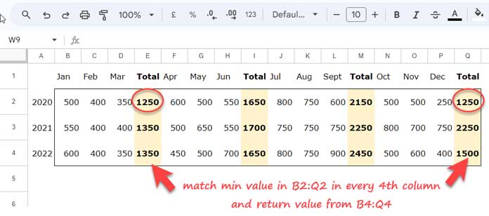
I want to use the INDEX MATCH function to find the minimum production in every fourth column (every quarter) in row 2 (year 2020) and return the corresponding quarter’s production in row 4 (year 2022).

We typically use MATCH to locate a value and INDEX to offset that result.

In the first example, we will see how to use the INDEX MATCH combination to find the minimum value in every nth column in Google Sheets and return the corresponding value in another row.

If there are multiple matching values, we can use the FILTER function to return all of them.

Once you’ve learned this technique, you can apply it to find the maximum value or any other specific value using INDEX MATCH Every nth Column in Google Sheets.

INDEX MATCH Minimum Value for Every Nth Column in Google Sheets

We will use the above table for the example. Here is the formula:

=ARRAYFORMULA(
     LET(
          f_row, B2:Q2,
          r_row, B4:Q4,
          n, 4,
          test, MOD(SEQUENCE(1, COLUMNS(f_row)), n),
          fnl, IF(test=0 ,f_row,),
          INDEX(r_row, 1, MATCH(MIN(fnl), fnl, 0))
     )
)

Where:

• f_row (find row): The range of cells in row 2 (B2:Q2) that contains the values to match.
• r_row (return row): The range of cells in row 4 (B4:Q4) that contains the values to return.
• n: The number of columns to skip between each match. For example, to find the minimum value in every other column, set n = 2.

We’ll cover the rest of the formula parts—test, fnl, and the INDEX MATCH Every nth Column in Google Sheets formula—in the anatomy section below.

When using the formula to INDEX MATCH the minimum value in every nth column, you only need to modify the three main arguments:

• Replace B2:Q2 with the row containing the values to match.
• Replace B4:Q4 with the row containing the values to return.
• Replace 4 with the number of columns to skip between matches.

Note: f_row and r_row must be of equal size.

Understanding the Formula: Anatomy of INDEX MATCH

The following MOD-based formula returns 0 in every fourth column:

=ARRAYFORMULA(MOD(SEQUENCE(1, COLUMNS(B2:Q2)), 4))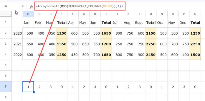

In our master formula, the relevant part is MOD(SEQUENCE(1, COLUMNS(f_row)), n). The name given to this expression is test.

Next, we use an IF logical test to return B2:Q2 if the test equals 0, or an empty string otherwise:

=ARRAYFORMULA(IF(B7:Q7 = 0, B2:Q2, ""))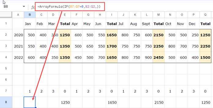

In the master formula, this is IF(test = 0, f_row, ""). The name given to this expression is fnl.

Finally, the INDEX MATCH Every nth Column in Google Sheets formula is:

=INDEX(B4:Q4, 1, MATCH(MIN(B8:Q8), B8:Q8, 0))

Or, in the master formula:

INDEX(r_row, 1, MATCH(MIN(fnl), fnl, 0))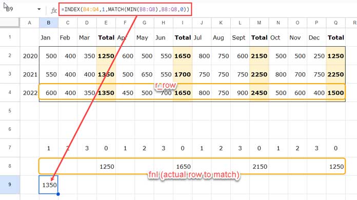

INDEX MATCH Maximum Value for Every Nth Column in Google Sheets

Using the same sample data, here is the formula to INDEX MATCH the maximum value in every nth (4th) column in Google Sheets:

=ARRAYFORMULA(
     LET(
          f_row, B2:Q2,
          r_row, B4:Q4,
          n, 4,
          test, MOD(SEQUENCE(1, COLUMNS(f_row)), n),
          fnl, IF(test=0, f_row,),
          INDEX(r_row, 1, MATCH(MAX(fnl), fnl, 0))
     )
)

The only difference is using MAX instead of MIN.

Handling Multiple Matches in Every Nth Column

The above formulas have a limitation: they cannot return multiple values.

For example, in the previous example, 1250 is the minimum value in B2:Q2. It appears in cells E2 and Q2. So, the corresponding values in B4:Q4 are 1350 and 1500.

The INDEX MATCH formula only returns 1350. To get all matching values, use FILTER:

=ARRAYFORMULA(
     LET(
          f_row, B2:Q2,
          r_row, B4:Q4,
          n, 4,
          test, MOD(SEQUENCE(1, COLUMNS(f_row)), n),
          fnl, IF(test=0, f_row,),
          FILTER(r_row, fnl = MIN(fnl))
     )
)

You can replace MIN with MAX to return all corresponding maximum values.

Using INDEX MATCH with Custom Criteria in Google Sheets

You’re not limited to minimum or maximum values. You can use any condition, including text criteria.

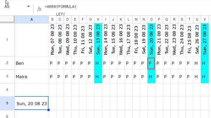
For example, to check if an employee was present (marked as “P”) on any Sunday and return the corresponding date:

=ARRAYFORMULA(
     LET(
          f_row, B2:V2,
          r_row, B1:V1,
          n, 7,
          test, MOD(SEQUENCE(1, COLUMNS(f_row)), n),
          fnl, IF(test=0, f_row,),
          INDEX(r_row, 1, MATCH("P", fnl, 0))
     )
)

To return multiple matches, replace the INDEX MATCH part with:

FILTER(r_row, fnl = "P")

Conclusion

An important aspect of the INDEX MATCH Every nth Column in Google Sheets formula is how the nth is counted.

For example, if nth = 4, the formula defaults to columns 4, 8, 12, 16, 20. What if you want to start at the first column instead (1, 5, 9, 13, 17)?

Modify the formula as follows:

MOD(SEQUENCE(1, COLUMNS(f_row), n), n)

This adjusts the starting point for every nth column.

Resources

• How to Sum Every Nth Row or Column in Google Sheets
• How to Highlight Every Nth Row or Column in Google Sheets
• How to Copy Every Nth Cell from a Column in Google Sheets
• Select Every Nth Column in Google Sheets Query – Dynamic Formula
• Delete Every Nth Row in Google Sheets (No Script Needed)
• How to Import Every Nth Row in Google Sheets
• Date Sequence Every Nth Row in Excel (Dynamic Array)