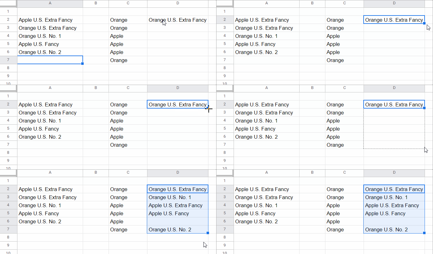
If you’ve ever used the FILTER function in Google Sheets, you know how powerful it is for narrowing down lists based on criteria. But what if the same criterion appears more than once, and you want a different result for each occurrence — like returning the first match for the first appearance, second match for the second appearance, and so on?
In this tutorial, you’ll learn how to index a filtered range in Google Sheets by combining INDEX, FILTER, and COUNTIF. This lets you dynamically return values from filtered results based on how many times a search key has appeared above — a technique especially useful when distributing matches across rows.
Introduction
In Google Sheets, filtering data and retrieving specific results is straightforward with FILTER. However, things get tricky when the same search key appears multiple times and you want to return progressively different results.
This tutorial shows how to:
- Filter a range by a key (with partial match)
- Return the first, second, third matching result as the key repeats
- Handle blank cells and errors gracefully
- Extend the method to multi-column datasets
In short, we’ll see how to index filtered range results by count of occurrence — without helper columns or scripting.
Sample Scenario and Goal
Let’s say you have a list of fruits with their quality grades in column A:
| A |
|---|
| Apple U.S. Extra Fancy |
| Orange U.S. Extra Fancy |
| Orange U.S. No. 1 |
| Apple U.S. Fancy |
| Orange U.S. No. 2 |
And in column C, you have a list of fruit names as your search keys:
| C |
|---|
| Orange |
| Orange |
| Apple |
| Apple |
| Orange |
The task is to search for each key in column A, and return a matching result for each row — but each time, return the next matching item. So:
- First
"Orange"→ returns first Orange in A - Second
"Orange"→ returns second Orange in A - Third
"Orange"→ returns third Orange in A

Index a Filtered Range by Occurrence Count – Drag-Down Formula
Let’s build this up step by step.
1. Filter Formula with Partial Match
Use the FILTER function with SEARCH to return all rows that contain the text in C2. In cell D2:
=FILTER($A$2:$A, SEARCH(C2, $A$2:$A))This will return all matches in A2:A where the value partially matches C2 (e.g., “Orange” matches “Orange U.S. No. 1”).
2. Count Occurrences Using COUNTIF
In cell E2, try:
=COUNTIF($C$2:C2, C2)This gives a running count of how many times the current value has appeared in column C up to that point.
This count will serve as the row offset for the INDEX function.
3. Combine with INDEX
Now combine FILTER and COUNTIF using INDEX, in D2:
=INDEX(
  FILTER($A$2:$A, SEARCH(C2, $A$2:$A)),
  COUNTIF($C$2:C2, C2)
)
This returns:
- The first match for the first occurrence
- The second match for the second occurrence
- And so on…
Copy this down for D2:D6.
4. Final Formula with Blank and Error Handling
To make it more robust:
=IF(C2="",,IFERROR(INDEX(
  FILTER($A$2:$A, SEARCH(C2, $A$2:$A)),
  COUNTIF($C$2:C2, C2)
)))- Prevents errors when there aren’t enough matches
- Skips blank search keys in column C
Try It Yourself
Want to see how the formula works in a live sheet?
This includes the drag-down formula, input data, and a working example.
Index a Filtered Range by Occurrence Count – Array Formula
If you prefer no drag-down, you can use an array formula version with MAP and LAMBDA:
=MAP(C2:C, LAMBDA(seq_,
  LET(
    ftr, FILTER(A2:A, SEARCH(seq_, A2:A)),
    IF(seq_="",,IFERROR(INDEX(ftr, COUNTIF(C2:seq_, seq_))))
  )
))
How it works:
MAPloops over each value in C2:CFILTERgets all matching rowsCOUNTIF(C2:seq_, seq_)returns the nth matchINDEXreturns that rowIFERRORhandles out-of-bounds and blank cases
Working with Multi-Column Data
If your original dataset spans multiple columns — say, A2:B with fruit name and quantity — you can adjust the formula:
=INDEX(
  FILTER($A$2:$B, SEARCH(C2, $A$2:$A)),
  COUNTIF($C$2:C2, C2)
)
This will return the full row — for example, both fruit and its quantity.
You can do the same in the array formula version by changing the FILTER range to A2:B.
Summary
With this approach, you’ve now learned how to:
- Index a filtered range in Google Sheets by the number of times a search key appears
- Use INDEX, FILTER, and COUNTIF together for progressive lookup
- Avoid errors and blanks
- Apply the formula to arrays and multi-column data
This method is ideal when:
- You need to distribute filtered results across rows
- You’re working with repeated search keys
- You want a clean, formula-only solution — no scripts, no helper columns


Your fastest responses always save my day. Thank you, Prashanth!
You are welcome!
Hi, Prashanth!
Sometimes the data stays in the proper rows, but sometimes it doesn’t.
Can you help me with the expected output in column F?
Thank you!
I found the following:
Range: A2:A
Search Keys: E2:E
The following formula in cell F2 partially matches E2 in A2:A and returns the first occurrence.
=IFERROR(INDEX(FILTER($A$2:$A,SEARCH(E2,$A$2:$A)),COUNTIF($E$2:E2,E2)))You are required to copy and paste it down. If the search key repeats, it will return the second occurrence, and so on.