How to Use IMPORTRANGE with Conditions in Google Sheets

You can’t directly use conditions within the Google Sheets IMPORTRANGE function. To apply conditions, you need to combine it with either the QUERY or FILTER function.

Which One to Choose?

Using QUERY

You can use IMPORTRANGE as the data source in QUERY.
It may be complex if you’re unfamiliar with the function, as literals can be confusing.
Supports case-sensitive filtering.

Using FILTER

To avoid multiple uses of IMPORTRANGE, wrap it in LET.
Use INDEX or CHOOSECOLS to select the column where conditions apply.
Case-insensitive.
Easier to specify conditions.
You may lose the header of the imported table, as FILTER might exclude it.

Example: Applying IMPORTRANGE with Conditions Using QUERY

Step 1: Importing Data

Assume the following sample data is in the source sheet, in the range A1:E10:

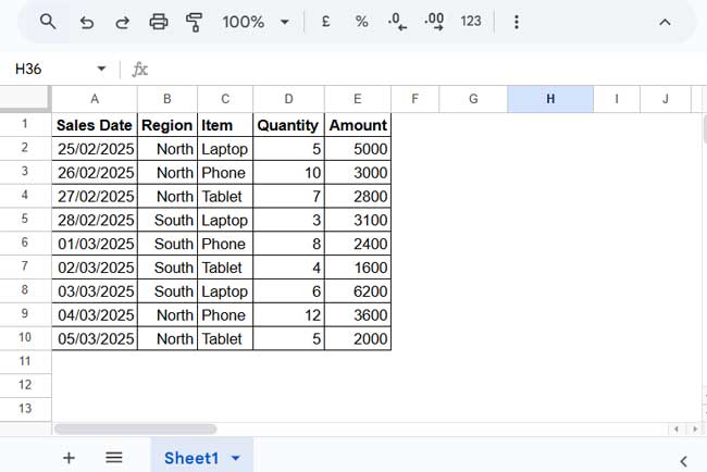
Example of using IMPORTRANGE with conditions in Google Sheets

In the destination sheet, use the following formula to import the data:

=IMPORTRANGE("https://docs.google.com/spreadsheets/d/1I62hdJ0mK5WhgXdoMWBfcAd-fFmN2KbwbSgdcNK2mes/edit?gid=0#gid=0", "Sheet1!A1:E10")

Step 2: Allowing Access

If you see a #REF! error, hover over it and click Allow Access to grant permissions.

Step 3: Applying Conditions

To filter this data using QUERY, apply the condition as follows:

=QUERY(IMPORTRANGE("https://docs.google.com/spreadsheets/d/1I62hdJ0mK5WhgXdoMWBfcAd-fFmN2KbwbSgdcNK2mes/edit", "Sheet1!A1:E10"), "SELECT * WHERE Col2='North'")

This formula filters the imported data where column 2 (Region) equals "North".

If you want to retrieve specific columns, modify the formula as follows:

=QUERY(IMPORTRANGE("https://docs.google.com/spreadsheets/d/1I62hdJ0mK5WhgXdoMWBfcAd-fFmN2KbwbSgdcNK2mes/edit?gid=0#gid=0", "Sheet1!A1:E10"), "SELECT Col1, Col2, Col5 WHERE Col2='North'")

By default, QUERY is case-sensitive. To make it case-insensitive, use:

=QUERY(IMPORTRANGE("https://docs.google.com/spreadsheets/d/1I62hdJ0mK5WhgXdoMWBfcAd-fFmN2KbwbSgdcNK2mes/edit", "Sheet1!A1:E10"), "SELECT * WHERE LOWER(Col2)='north'")

This is one way to use IMPORTRANGE with conditions.

Example: Applying IMPORTRANGE with Conditions Using FILTER

Using FILTER with IMPORTRANGE was previously inefficient since IMPORTRANGE had to be used multiple times—both in the range and condition parts. However, with the LET function, this has become much simpler.

=LET(qry, IMPORTRANGE("https://docs.google.com/spreadsheets/d/1I62hdJ0mK5WhgXdoMWBfcAd-fFmN2KbwbSgdcNK2mes/edit", "Sheet1!A1:E10"), FILTER(qry, CHOOSECOLS(qry, 2)="North"))

Explanation:

IMPORTRANGE fetches data and is stored in qry using LET.
FILTER(qry, CHOOSECOLS(qry, 2)="North") filters the Region column (Column 2) for "North".

To extract specific columns, modify the formula as follows:

=LET(qry, IMPORTRANGE("https://docs.google.com/spreadsheets/d/1I62hdJ0mK5WhgXdoMWBfcAd-fFmN2KbwbSgdcNK2mes/edit", "Sheet1!A1:E10"), FILTER(CHOOSECOLS(qry, 1, 2, 5), CHOOSECOLS(qry, 2)="North"))

CHOOSECOLS(qry, 1, 2, 5) extracts columns 1, 2, and 5.
The condition CHOOSECOLS(qry, 2)="North" applies the filter to column 2 (Region).

This is another way to use IMPORTRANGE with conditions in Google Sheets.

Additional Resources

58 COMMENTS

Liz F. February 10, 2023 At 9:07 pm

Hi! I am only able to get the first row of data to appear in the new spreadsheet, none of the other data is being transferred.

=QUERY(IMPORTRANGE("URL","codes!B2:E200"),"SELECT Col1,Col2, Col3, Col4 where lower(Col1)='y'",1)

Thanks for your help!

- Prashanth February 11, 2023 At 9:01 am
  
  Hi, Liz F.,
  
  The formula seems correct to me and works on my test sheet.
  
  Try replacing lower(Col1)='y' with lower(Col1) starts with 'y'
  
Shawna February 8, 2023 At 5:05 am

Hey Prashanth,

I am trying to use the following code, but I am still getting an Error: Unable to parse query string for Function QUERY parameter 2: NO_COLUMN: Col7

=QUERY(IMPORTRANGE("URL","Sheet1!E2:E2000"),"where Col7='YouTube'")

- Prashanth February 8, 2023 At 10:17 am
  
  Hi, Shawna,
  
  You are importing only one column that is numbered Col1, not Col7.
  
Jennell V. December 10, 2022 At 12:27 am

Hi Prashanth,

Thank you for this tutorial. I am hoping you are still checking comments. I was able to get this to work perfectly using the formula below:

=QUERY(IMPORTRANGE("URL","2023 DATA COLLECTION!A3:Y7"),"where Col1='Bob.S.'")

Now, I am trying to find a way to select Bob.S. in a drop down (data validation) and have the information import from the main data sheet. Can you tell me if this is possible.

Thank you for being a such great resource.

- Prashanth December 10, 2022 At 2:59 pm
  
  Hi, Jennell V.,
  
  If G2 contains the drop-down, then the last part of your formula will be as follows.
  
  "where Col1='"&G2&"'")
  
  To learn, please search the term “Literals” within this tutorial.
  
Jen Thatcher October 8, 2021 At 2:25 am

I’ve just spent a while watching tutorials but still can’t figure out why I am getting an “Unable to parse query string for Function QUERY parameter 2: NO_COLUMN: Col2” with this formula:

=QUERY(IMPORTRANGE("URL", "Sheet1!U6:U4426"), "where Col2='Set Value'")

- Prashanth October 8, 2021 At 12:31 pm
  
  Hi, Jen Thatcher,
  
  It’s because there is only one column in your imported data.
  
Bambi September 19, 2021 At 6:23 pm

Hello, Thank you for the lesson. It is almost working, but it is importing the first row in my source range (A3) even though it doesn’t meet my criteria- all other rows are correct. Here is my formula:

=QUERY(IMPORTRANGE("URL","Sheet1!A3:P"),"where Col3='8/313'")

- Prashanth September 20, 2021 At 9:28 am
  
  Hi, Bambi,
  
  Query treats it as the Header.
  
  Try this formula instead.
  
  =QUERY(IMPORTRANGE("URL","Sheet1!A3:P"),"where Col3='8/313'",0)
  
Ahmad Akmal September 14, 2021 At 5:56 am

Hi Mr. Prashanth, I am glad I read your post here.

The Importrange is working like a charm. Unfortunately, the Query which comes after didn’t work.

My example:

=IMPORTRANGE("https://docs.google.com/spreadsheets/d/xx/edit#gid=xx","BA 111!C6:O140"),"where Col4='TIADA'")

- Prashanth September 14, 2021 At 3:16 pm
  
  Hi, Ahmad Akmal,
  
  You have not used the Query function in your formula.
  
  E.g.
  
  =query( IMPORTRANGE("https://docs.google.com/spreadsheets/d/xx/edit#gid=xx","BA 111!C6:O140"), "where Col4='TIADA'" )
  
mohd faizal che hussin July 29, 2021 At 11:00 am

Hi All,

Used below formula for my work:

=IMPORTRANGE("URL_here","d9:d12")

Any step to change the output to horizontal?

- Prashanth July 29, 2021 At 12:39 pm
  
  Hi, mohd faizal che hussin,
  
  Try this.
  =transpose(IMPORTRANGE("URL_here","d9:d12"))
  
Paul Salcedo February 10, 2021 At 6:48 am

Hi Prashanth,

I’ve learned so much from your articles, so hats off.

However, my problem now is to combine the AND function with IMPORTRANGE.

I am trying to import the data from a source workbook on the condition that a cell in the destination workbook contains my name. Is this possible?

If not, could you suggest an add-on that executes this task? Here is the formula:

=AND(IMPORTRANGE("12hHtTrXsL1pL_Fz7dH-ZejG4srs8DSTfxmKUAeEfh64","02-02-2021!D276:$K"), $B:B="Paul Salcedo",)

Also, let me know if there’s anything wrong with this formula.

Paul

- Prashanth February 11, 2021 At 9:42 am
  
  Hi, Paul Salcedo,
  
  It is possible. I am unable to write the formula because you have not specified the cell that contains your name in the destination sheet. Also, in the source, which column contains your name.
  
  I assume you want to import the data if column 2 (column B) in your source contains your name.
  
  So the formula must be something like this-
  
  =Query(IMPORTRANGE("12hHtTrXsL1pL_Fz7dH-ZejG4srs8DSTfxmKUAeEfh64","02-02-2021!A276:K"),"Select * where Col2='Paul Salcedo'")
  
  This may help you – How to Use Query with Importrange in Google Sheets.
  
Brooke February 3, 2021 At 7:28 am

Hi, I am trying to do this exact thing but I want to translate this data between different tabs in one Google Sheet but only one column of the information if a different column is a certain value.

So if column D in sheet 1 says “Jane Doe”, I want it to populate the information from column B into sheet 2

B | C | D | E
Frog | Test | Jane Doe | Blue
Cat | Test | Jane Doe | Orange
Bear | Test | John Doe | Yellow

So I want when it says Jane Doe to populate the animals into a column on sheet 2 and nothing else.

- Prashanth February 4, 2021 At 9:45 am
  
  Hi, Brooke,
  
  In Sheet2, try this formula.
  
  =query(Sheet1!B1:E,"Select B where D='Jane Doe'")
  
  In this formula, if the sheet name is “Sheet 1” not “Sheet1”, then use it as below.
  
  =query('Sheet 1'!B1:E,"Select B where D='Jane Doe'")
  
Owen October 13, 2020 At 9:26 pm

Thank you so much for posting this. I have spent all afternoon trying to figure it out. I don’t know why Google has not made it clearer that the syntax is different when IMPORTRANGE is used.

- Prashanth October 16, 2020 At 10:34 am
  
  Hi, Owen,
  
  Not only IMPORTRANGE. If you use an expression as the Query ‘data’ (please refer to the syntax below) then you should follow a different formula approach.
  
  Syntax: QUERY(data, query, [headers])
  
  Normal data range can also be changed as an expression by putting curly brackets around.
  
  Examples:
  
  =query(A1:B,"Select * where A contains 'SEO'")
  
  Which can be replaced by;
  
  =query({A1:B},"Select * where Col1 contains 'SEO'")
  
Louis Lee August 20, 2020 At 10:08 am

Hi,

May I know does a way to change the condition by specific tab sheets?

I have the main database that will assign people for some specific work. Then this work details will be imported to that assigned people spreadsheets workbook by using queryImportRange formula.

However, instead of using where Col6 = 'Worker Name', does I able to auto change this to query the value by using my tab sheets name?

Cause I have a lot of spreadsheets, I wish I don’t have to copy the formula and change the condition one by one.

Original Formula:

=QUERY(IMPORTRANGE("URL","assigned!B2:P"),"select Col1,Col2,Col3,Col4,Col5,Col6,Col7,Col8,Col9,Col10,Col11 where (Col13 = ' Louis')")

- Prashanth August 21, 2020 At 10:22 am
  
  Hi, Louis Lee,
  
  I do have a workaround formula. The formula takes three blank cells in each sheet as helper cells (you can spare the top row for that). Also, there is one more constraint that it updates the tab names similar to volatile functions like now(), I mean once you enter any value in any cell.
  
  I’ll post it soon and let you know by sharing the link below.
  
- Prashanth August 25, 2020 At 1:56 pm
  
  Hi, Louis Lee,
  
  Please see my new post – Current Sheet Name as the Criterion in Google Sheets Formulas (Workaround),
  
  I was super busy, sorry for the delay in getting back.
  
Fariya Adnan August 9, 2020 At 5:45 pm

Can anyone tell me what’s wrong with this?

=QUERY(IMPORTRANGE(“URL″,”Sheetname!F2:F”),”where Col6=’Opportunity'”)

- Prashanth August 11, 2020 At 11:02 am
  
  Hi, Fariya Adnan,
  
  The issues are with the double as well as single quotes. It should be " for double quotes and ' for single quotes.
  
Joyce July 21, 2020 At 3:06 am

How do I take selected columns with a Where condition? The following two scripts work separately but I cannot have both into one script?

=Query(importrange("xxxxx","'SheetName'!$A:$U"),"SELECT Col6,Col9,Col10",1) =Query(importrange("xxxxx","'SheetName'!$A:$U"),"where Col17='Test'")

- Prashanth July 21, 2020 At 10:01 am
  
  Hi, Joyce,
  
  It should be like this.
  
  =Query(importrange("URL","'SheetName'!$A:$U"),"SELECT Col6,Col9,Col10 where Col17='Test'",1)
  
  The above Query is case sensitive. Use SMALL() to make it case insensitive.
  
  =Query(importrange("URL","'SheetName'!$A:$U"),"SELECT Col6,Col9,Col10 where lower(Col17)='test'",1)
  
Mark Larbalestier February 27, 2020 At 11:19 pm

Hi,

Sorry to ask but this looks like the closest possible thread to help me.

I have Google Forms answers transferring to Google Sheets and then coded to log as an easy to read table. I am now looking to see if I can get an automatic transfer of data to a “Monthly” Sheet.

I.e all answers are listed by date on one Sheet, can I set formula to move January responses to January tab, February responses to February tab, etc, etc, etc…

At present, I am cutting and pasting data from the table to individual sheets but would prefer, if it could do it for me!

Thanks

Mark

- Prashanth February 28, 2020 At 8:58 am
  
  Hi, Mark Larbalestier,
  
  I assume the first tab (tab name, for example, is “Master”) contains the data being collected through Google Forms.
  
  In the same file, in the second tab (tab name, for example, is “Jan”), enter the below Query.
  
  =query('Master'!A1:Z,"Select * where month(A)=0")
  
  For ‘Feb’ tab,
  
  =query('Master'!A1:Z,"Select * where month(A)=1")
  
  For ‘Mar’ tab,
  
  =query('Master'!A1:Z,"Select * where month(A)=3")
  
  Month number 0 is for Jan, 1 is for Feb and so on.
  
  I have considered that column A contains the dates. If some other column contains the dates, for example, column B, then change month(A) to month(B).
  
  - Mark Larbalestier February 28, 2020 At 10:14 pm
    
    This worked perfectly on my test sheet but wouldn’t work on the actual workbook I need it for some reason.
    
    I’m not sure if its because the responses have already been coded into a table on Tab 2 although I copied+pasted your query formula above.
    
    If this makes sense, my responses are on Tab 1 named ‘Form Responses’. Tab 2 has a table formed using Coding and this is called ‘AV12 Log’. Tab 3 should be the query tab looking for the monthly requirement. Have I missed something?
    
    - Prashanth February 29, 2020 At 9:09 am
      
      Hi, Mark Larbalestier,
      
      There may be two possible reasons.
      
      1. The date column may be formatted as text.
      2. Improper sheet name, for example,
      
      =query(AV12 Log!A1:Z,"Select * where month(A)=0")
      
      In this, the sheet name must be within single quotes as;
      
      =query('AV12 Log'!A1:Z,"Select * where month(A)=0")
      
      If your sheet doesn’t contain any personal/confidential info, you can share it in the ‘VIEW’ mode so that I can check the cause of the problem. I won’t publish the sheet link.
      
Matt January 22, 2020 At 8:14 am

Hey there, this is amazing. Thank you so much. One issue is for some reason when I have about 130 cells in a row of phone numbers then it freaks out and starts piling data in the first row. Kinda hard to explain, but basically when I get rid of the phone number column in my spreadsheet, then it works fine. Any ideas?

- Prashanth January 22, 2020 At 11:05 am
  
  Hi, Matt,
  
  Format the column which contains the phone numbers to ‘text’ by going to the Format menu, Number > Plain text.
  
  See if that works?
  
  - Matt January 23, 2020 At 12:02 am
    
    Wow. Absolutely amazing. Thanks! This has seriously helped me so much.
    
Ryan October 21, 2019 At 11:27 pm

Thanks for the great help. I was wondering how you’d filter for two different queries. Suppose you wanted data from two different columns…Maybe the first is “where Col1=’Safety Helmet'” and Col2=’Medium Size”…How would you do that?

Thanks.

- Prashanth October 22, 2019 At 9:17 am
  
  You are on the right track.
  
  Instead of this Query Importrange;
  
  =QUERY(IMPORTRANGE("URL","SHEET1OFTESTA!A1:G9"),"where Col1='Safety Helmet'")
  
  Use this one;
  
  =QUERY(IMPORTRANGE("URL","SHEET1OFTESTA!A1:G9"),"where Col1='Safety Helmet'and Col2='Medium Size'")
  
Joydev Chakraborty October 3, 2019 At 9:55 pm

Hi Sanjeev, I have a question. If I want to count no. of times a particular text string appeared in column 4, named as “Column Name” in the source spreadsheet and project that in the spreadsheet I am currently working on, how do I do that? I tried the following query but it returns “0”, but there are text strings in the source spreadsheet.

=countif(IMPORTRANGE("Enter URL Here", "Sheet 1!D:D"), "where Column Name= '2 - Review'")

Please help.

- Prashanth October 4, 2019 At 10:33 am
  
  Hi, Joydev Chakraborty,
  
  You can use the COUNT function within the SQL similar Query function in Sheets. You can try the formula as below.
  
  =IMPORTRANGE("Enter URL Here", "Sheet 1!D:D"), "Select Col1, Count(Col1) where Col1='2 - Review' group by Col1")
  
  Best,
  
Sanjeev Kaushik July 30, 2019 At 1:52 am

What would be the query if I want data to be returned for “Safety Helmet” and “Illuminated Jacket”.

Will it differ in case there is a digit or a number like 763 and 957 in place of Safety Helmet and Illuminated Jacket.

- Prashanth July 30, 2019 At 9:09 am
  
  Hi, Sanjeev,
  
  For using multiple number criteria in the same column, use the logical operator OR in Query as below.
  
  =QUERY(Importrange formula here,"where Col1=763 or Col1=957")
  
  When the criteria are strings, then enclose each criterion within single quotes.
  
  Eg. =QUERY(Importrange formula here,"where Col1='Illuminated Jacket' or Col1='Safety Helmet'")
  
Mari July 11, 2019 At 2:08 am

What if the filtering criteria are outside my range? For example, if I want to import only the column A into a new sheet but the filtering criteria (in this case, a TRUE/FALSE string) is in column C, could I select a new range out of the original sheet for the query portion? Or are there alternative functions that would allow me to do something similar? The end goal is to import column A where the corresponding value in column C is false.

- Prashanth July 11, 2019 At 12:01 pm
  
  Hi, Mari,
  
  See this example formula.
  
  =query(IMPORTRANGE("enter URL here","Sheet1!A1:C"),"Select Col1 where Col3=TRUE")
  
  Best,
  
Sarah June 14, 2019 At 12:55 am

I’m new to more advanced uses of Google Sheets and found this very useful.

I’ve just spent a while watching tutorials but still can’t figure out why I am getting an “Unable to parse query string for Function QUERY parameter 2: NO_COLUMN: COL4” with this formula:

=QUERY (importrange ("URL", "Riding List!A1:K500"), "WHERE COL4 = 'Confirmed'")

- Prashanth June 14, 2019 At 9:32 am
  
  Hi, Sarah,
  
  You were very close. Just change COL4 to Col4.
  
  Best,
  
  Prashanth KV
  
  - Yatrik2 July 9, 2019 At 7:12 am
    
    Hi Prashanth,
    
    First, thank you for the lesson. Very helpful.
    
    I had the same problem and it was solved by changing COL1 to Col1. Perhaps you can revise your tutorial and change it there too.
    
    - Prashanth July 9, 2019 At 8:40 am
      
      Hi, Yatrik2,
      
      I didn’t realize that the error was happening from my formula itself. I have just corrected that typo.
      
      Thanks for notifying me.
      
Maurice Bell June 4, 2019 At 8:37 pm

Wondering with I’m getting an error (formula parse error) when following your example?

=QUERY(IMPORTRANGE("https://docs.google.com/spreadsheets/d/19CtkZXfr-UpTX9qkgAOl95Ci4QGU-u3GmzqOzj1zM7s/edit#gid=1971556446","Sheet1ofTimecard!A1:G9″),"where Col2='Keesh Pinerro'")

- Prashanth June 5, 2019 At 9:36 am
  
  Hi, Maurice Bell,
  
  This could be due to your Spreadsheet Setting (File > Spreadsheet settings).
  
  If that setting is pointing to any EU countries, then you must replace the comma , before the “where…” clause in your formula to a semicolon ;
  
  Hope this helps.
  
  Best,
  
  - Isaac Francisco June 12, 2019 At 9:03 pm
    
    I had the same problem but was able to resolve it by updating the " (double quotes)
    check this part:
    "Sheet1ofTimecard!A1:G9″
    
    Update that and that should fix your error.
    
    - Prashanth June 13, 2019 At 9:22 am
      
      Hi, Isaac,
      
      I have just edited this post. The formula was not entered as a code for highlighting a certain part of it.
      
      Thanks.
      
  - Prafull Jaiswal June 25, 2019 At 4:03 pm
    
    Hi Prasanth,
    
    I am also facing the same issue. Below mentioned are the details.
    
    Formula used =Query(importrange("URL","Open Positions!A1:AG1972"),"Where COL4='Abin Thomas'")
    
    Error –
    
    “Unable to parse query string for Function QUERY parameter 2: NO_COLUMN: COL4”
    
    Spreadsheet Setting – Pointing to the US.
    
    Request your help to resolve this.
    
    - Prashanth June 26, 2019 At 8:34 am
      
      Hi, Prafull Jaiswal,
      
      Please change COL4 to Col4.
      
      Best,
      
Ben April 6, 2019 At 4:38 am

Hi,

I just want to ask, Can I combine the function IFS statement and importrange function? If so could you please send me an example.

Cheers,

- Prashanth April 6, 2019 At 9:10 am
  
  Hi, Ben,
  
  Please let me know the purpose. So that I can give you a correct reply.
  
Paula H. December 29, 2018 At 10:38 am

Hi,

Thank you so much for this. I have been searching high and low and finally found this formula and was able to understand it from your tutorial.

I have one question, how would I get the data to copy to another sheet in the same document and then delete the info from the original sheet (which is from a google form)? Hope this makes sense.

- Prashanth December 30, 2018 At 11:33 am
  
  Hi,
  
  Use the function Query or Filter to (conditionally) copy the data to another tab. For example Form data in Sheet1 to Sheet2. Then select the entire data range in Sheet2, right-click to copy and again right-click > Paste Special > Values only.
  
Ankush kumar October 16, 2018 At 3:04 pm

I want to learn Importrange with Query.

- Prashanth December 1, 2018 At 10:19 am
  
  Hi, Ankush,
  
  Sorry for the late reply. Your request was in my mind. See the new tutorial based on your request.
  
  https://infoinspired.com/google-docs/spreadsheet/query-with-importrange-in-google-sheets/
  
  See if that helps?
  Cheers!