How to Use the IMPORTHTML Function in Google Sheets

The IMPORTHTML function helps import tables and ordered or unordered lists from web pages into Google Sheets.

When you copy-paste data from a table found on any web page into Google Sheets, it may lose its tabular form. As a result, you might need to apply data manipulation techniques to reformat it back into a table, which can be time-consuming. To solve this, you can use the IMPORTHTML function in Google Sheets.

When the data on the external web page updates, the same changes will automatically reflect in the IMPORTHTML imported data.

For example, when you see a table on a blog page, such as in a tutorial, and you want to use that table in your sheet for testing purposes, you can use the IMPORTHTML function for that.

Example:

=IMPORTHTML("https://infoinspired.com/google-docs/spreadsheet/how-to-highlight-vlookup-result-value-in-google-sheets/", "table", 1)

Syntax and Arguments

Syntax:

IMPORTHTML(url, query, index)

Arguments:

url: The URL of the HTML page containing the table or list to import. It must be enclosed within double quotes when hardcoding in the formula.
query: This parameter supports one of two arguments: “list” or “table”.
index: The index of the table or list to import. The table or list number starts at 1. If a webpage contains multiple tables or lists, specifying 5 will import the fifth table or list, depending on the query argument.

In summary, with the help of the IMPORTHTML function, you can import the following:

Tables: Data structured in rows and columns within <table> tags.
Lists: Data presented as sequential items, either ordered (<ol>) or unordered (<ul>).

Examples of Using the IMPORTHTML Function in Google Sheets

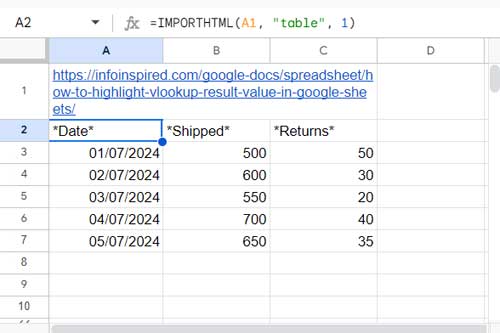
Say you’re reading a blog post about highlighting VLOOKUP results on a website. The post has a table demonstrating the process. You can use IMPORTHTML to import that table directly into your Google Sheet for reference or testing purposes.

Here’s an example formula that imports the first table from this webpage:

Importing a Table:

IMPORTHTML Function to Import a Table in Google Sheets

Steps:

Enter the following URL in cell A1:
https://infoinspired.com/google-docs/spreadsheet/how-to-highlight-vlookup-result-value-in-google-sheets/
In cell A2, enter the following IMPORTHTML formula:
=IMPORTHTML(A1, "table", 1)
This will import the first table on the page. If you look at the page, you will see that there are two tables.
If you specify 3 as the index number, the formula will return #N/A since there are only two tables on the webpage.
If you omit the index or specify 0, the formula will return the first table.

Importing a List:

IMPORTHTML Function to Import a List in Google Sheets

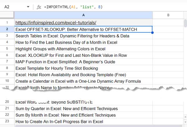
Enter the following URL in cell A1:
https://infoinspired.com/excel-tutorials/
In cell A2, use the following formula to import a list of my Excel tutorials available on that page:
=IMPORTHTML(A1, "list", 8)

Note:

IMPORTHTML is best for tabular data. Its performance and reliability with complex lists may be inconsistent.

Finding List or Table Number for IMPORTHTML Function

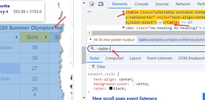
To find the table number on a webpage for use with the IMPORTHTML function in Google Sheets, follow these steps on Google Chrome:

Navigate to the webpage containing the table you want to import.
Right-click anywhere on the page and select “Inspect“.
Click on the Elements tab in the developer tools to view the HTML structure.
Press Ctrl+F (Windows) or Command+F (Mac) to open the search field.
In the search field, enter <table> to find tables.
Press the Enter key to highlight the search results in the HTML structure.
Count each occurrence until you find your desired table. Use this number as the index in the IMPORTHTML function.

This method is not ideal for locating lists due to the <ol> and <ul> tags. For lists, follow these steps:

Right-click on the desired list and select “Inspect“.
Manually count the number of <ol> and <ul> tags preceding the one you want to import.
The count you arrive at is the index number for your IMPORTHTML function.

While the provided method works for simple lists, specialized tools might be needed for complex websites.

Additional Notes

You may want to remove columns or rows from the imported data. For that, you can use the ARRAYCONSTRAIN, CHOOSECOLS, CHOOSEROWS, or QUERY functions.

I recommend using QUERY as it can identify the header row in the imported table and offset rows from the beginning.

Select Specific Columns:

=QUERY(IMPORTHTML(A1, "table", 1), "SELECT Col1, Col3")

Offset Rows:

=QUERY(IMPORTHTML(A1, "table", 1), "SELECT * OFFSET 2")

This skips the first two rows.

Limit Rows:

=QUERY(IMPORTHTML(A1, "table", 1), "SELECT * LIMIT 5")

This limits the output to 5 rows.

Resources

Here are some related Google Sheets resources.

23 COMMENTS

Dhiru March 20, 2023 At 5:56 pm

How to Importhtml table data from date ranges?

I want only dates between 25 to 31. Data tables have multiple months and multiple years.

- Prashanth March 20, 2023 At 7:05 pm
  
  Hi, Dhiru,
  
  The returned dates might be text formatted. So without seeing the data, I can’t suggest a formula.
  
  Please share a copy of your Sheet so that I can further assist.
  
Sneha December 15, 2021 At 2:02 pm

Hi Prashanth!

Once again, thank you for your tutorial.

I will need a minor variation in the above formula.

I have a list of 10 hyperlinks in column B. Each link has a table with five rows and three columns.

How do I manipulate the above formula so that I can extract all the 50 rows (i.e., five rows per entry, 5*10=50 rows)?

Thanks in advance!

- Prashanth December 16, 2021 At 8:54 am
  
  Hi, Sneha,
  
  Here is an example with three tables.
  
  ={ IMPORTHTML(B2,"table",1); IMPORTHTML(B3,"table",1); IMPORTHTML(B4,"table",1) }
  
Roycey June 8, 2020 At 8:25 pm

Thank you. The date in this URL:

=IMPORTHTML("URL;begindate=6/8/2020","table",2)

is actually the “Ex-Date” listed on the table. As I mentioned earlier, I have to manually change the date in the URL to the date after tomorrow in order to bring the table on which the “Ex-Date” is the date after tomorrow.

I used this new formula:

=IMPORTHTML("URL;begindate="&today()+2,"table",2)

but the new formula imports the table in which the Ex-Date is today date – not the date after tomorrow. Any clue?

Roycey June 8, 2020 At 10:28 am

Hello Prashanth,

I used this formula to import a table into my google sheets.

=IMPORTHTML("URL_Here;begindate=6/8/2020","table",2)

There is a date (6/4/2020) in the URL that I have to change every day manually to update the table to the date after tomorrow. Is there a way to change the date in the URL to the date after tomorrow automatically?

- Prashanth June 8, 2020 At 3:26 pm
  
  Hi, Roycey,
  
  In the below formula you can control the date by changing the formula part today()+2.
  
  =IMPORTHTML("URL_Here;begindate="&today()+2,"table",2)
  
  Best,
  
Tommy Sosa January 15, 2020 At 12:09 am

Hello Prashanth,

Thank you very much for the tutorial. I found it very informative.

I am currently receiving this error message “Resource at URL contents exceeded maximum size”. I even receive this error message after trying to specify query and filter parameters. By chance do you know what the size limitations are? Or perhaps a workaround to this error message?

Thank you in advance for any and all help.

- Prashanth January 15, 2020 At 8:39 am
  
  Hi, Tommy Sosa,
  
  I have no idea about that. Maybe something related to the source table.
  
shahaji shinde September 29, 2019 At 6:29 am

Hi Prashant,

Thanks for the article.

Need your support to address the below issue.

I have created a script to download and update the option chain at every 5 min.

The script runs every 5 mins but most of the time data is Old, how can I resolve this.

- Prashanth September 29, 2019 At 8:44 am
  
  Hi, Shahaji,
  
  Sorry to say, I’m not familiar with Google AppScript.
  
  Best,
  
Eliran Cohen August 10, 2019 At 10:13 pm

Hey, thanks for the article!

I’m trying to convert that page into a sheet with no success, any idea what I’m doing wrong?

=IMPORTHTML("https://crates.co/crate/spotify-labels/4720/feed","table",1)

Thanks!

Crusader April 20, 2019 At 6:19 am

Thank you for the article. How can I import the date to the right of “Earnings Date” into Google Sheets from the following website:

https://www.cnbc.com/quotes/?symbol=fl&qsearchterm=fl

Afzal February 18, 2019 At 2:40 am

Hello Prashanth,

I am trying to fetch the table and it is working fine but don’t know how to select the timeframe in the query.

Please can you have a look on this:

“https://www.investing.com/technical/pivot-points”

- Prashanth February 18, 2019 At 12:53 pm
  
  Hi, Afzal,
  
  I did check that. But that is not ‘possible’ with IMPORTHTML. I have seen some discussion on the web related to the same question. Please check this.
  
  stackexchange.com
  
  Best
  
Greg February 6, 2019 At 8:42 pm

Hey, maybe you can help, I’m trying to get the days, hours and minutes from this website.

“https://www.cmegroup.com/trading/interest-rates/countdown-to-fomc.html”

But I don’t think its a list or a table, any suggestions?

- Prashanth February 7, 2019 At 2:30 pm
  
  Sorry! It seems a count down timer. No way to import this using IMPORTHTML.
  
Dennis May 15, 2018 At 12:12 am

I have problems using select rows.
I have this

=IMPORTHTML("https://tweakers.net/pricewatch/1129515/nzxt-n7-z370-wit.html";"table";3)

That works, but now I want column 1 row 1 and column 4 row 1.

=query(IMPORTHTML(“https://tweakers.net/pricewatch/1129515/nzxt-n7-z370-wit.html”,”table”,2),”Select Col1,Col4″)

It does not work. Is it also possible to make it grab column 1 row 1 and column 4 row 1?

- Prashanth May 15, 2018 At 11:12 am
  
  Hi Dennis,
  
  You can do that.
  
  I think there is a typo in your second formula with the table number. OK let’s leave that aside.
  
  You can use the Query limit clause in this case.
  
  =query(IMPORTHTML("https://tweakers.net/pricewatch/1129515/nzxt-n7-z370-wit.html","table",3),"Select Col1,Col4 limit 1")
  
  Hope this may help.
  
AJAY May 14, 2018 At 4:52 pm

Please tell me how to fetch full table having more than 50 rows. I can fetch only the first 25 rows displayed on url webpage and remaining rows of table on same url ….i m unable to fetch using IMPORTHTML.

- Prashanth May 14, 2018 At 5:18 pm
  
  Hi Ajay,
  
  I didn’t face any such issues so far.
  The problem may be associated with webpage you are using.
  I’ve sent a mail to you. If possible share me the link. So that I can test it.
  
  Thanks.
  
Prashanth May 4, 2018 At 8:41 am

Hi Arun,
The fetched data will be auto updating based on the source.
We can’t set any intervals.

Arun May 3, 2018 At 5:21 pm

HI,

Thank you for the article above. It helped to create a google sheet to download the futures prices from NSE India website.
Can you also advise as to how to fetch the data at regular interval from the nse web site in this google sheet?

Thanks