An array result means a result that spans across a range instead of staying within a single cell. In some scenarios, we can use the IFS function to return an array in Google Sheets—yes, even though it’s not as flexible as IF.

To evaluate multiple conditions (criteria), we commonly use IF, SWITCH, or IFS. Of these, IF is the most popular but requires nesting (multiple IFs inside one another), which can quickly get messy.

The other two functions, SWITCH and IFS, are easier to read than nested IFs. While both can return array results, only IFS typically requires wrapping with ARRAYFORMULA. However, both functions fall short when asked to return multi-cell arrays from a single condition or when the condition and result ranges are mismatched.

In this post, I’ll explain how to use the IFS function to return an array/range result in Google Sheets. And if IFS doesn’t work for your case, I’ll show you a clean alternative that does.

Of course, consider using an IFS alternative only if nested IFs become too complex to write or maintain.

IFS Function to Return a Result in a Range in Google Sheets

Let’s explore two examples:

1. A working example of how to use the IFS function to return an array result in Google Sheets.
2. A case where IFS fails to return an array—and what to use instead (hint: IF or VLOOKUP can help).

Example: IFS Function That Returns an Array Result

Straight to the formula.

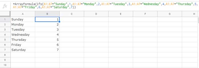
Let’s say you have the days of the week listed in cells A1:A7:

Sunday  
Monday  
Tuesday  
Wednesday  
Thursday  
Friday  
Saturday

Now you want to assign numbers to each day—1 for Sunday, 2 for Monday, and so on.

Here’s a working IFS array formula:

=ArrayFormula(IFS(
   A1:A7="Sunday", 1,
   A1:A7="Monday", 2,
   A1:A7="Tuesday", 3,
   A1:A7="Wednesday", 4,
   A1:A7="Thursday", 5,
   A1:A7="Friday", 6,
   A1:A7="Saturday", 7
))

This will return an array result in the adjacent column, one number for each corresponding day.

Handling IFS When a Condition Fails

There’s one catch. If any of the cells in A1:A7 are blank (or don’t match any condition), the formula will return a #N/A error. That’s because, unlike IF, the IFS function doesn’t have a value_if_false argument.

To fix this, you can add a fallback condition like this:

=ArrayFormula(IFS(
   A1:A7="Sunday", 1,
   A1:A7="Monday", 2,
   A1:A7="Tuesday", 3,
   A1:A7="Wednesday", 4,
   A1:A7="Thursday", 5,
   A1:A7="Friday", 6,
   A1:A7="Saturday", 7,
   1=1, "?"
))

Just replace the question mark ("?") at the end with your preferred fallback value.

• If it’s a string, keep it in double quotes.
• If it’s a number, you can drop the quotes.
• For dates or times, use DATE() or TIME() functions accordingly.

Example with a date fallback:

=ArrayFormula(IFS(
   A1:A7="Sunday", 1,
   A1:A7="Monday", 2,
   A1:A7="Tuesday", 3,
   A1:A7="Wednesday", 4,
   A1:A7="Thursday", 5,
   A1:A7="Friday", 6,
   A1:A7="Saturday", 7,
   1=1, DATE(2019, 8, 28)
))

Want a simpler solution? Here’s the same logic using SWITCH:

=SWITCH(A1:A7,
   "Sunday", 1,
   "Monday", 2,
   "Tuesday", 3,
   "Wednesday", 4,
   "Thursday", 5,
   "Friday", 6,
   "Saturday", 7,
   ""
)

But note: SWITCH doesn’t support comparison operators like <, >, or = within its arguments.

Where the IFS Function Fails to Return a Range Result

Let’s look at a case where the IFS function cannot return an array result.

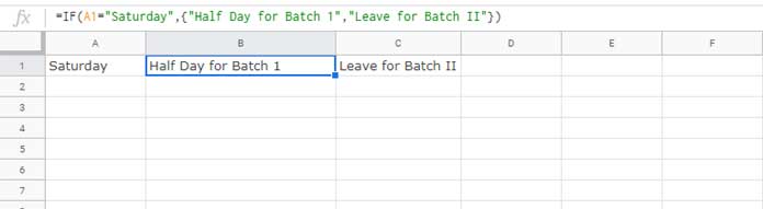
Say you have one value to evaluate (e.g., cell A1 has "Saturday") and you want to return two values if it matches.

Here’s an IF formula that works:

=IF(A1="Saturday", {"Half Day for Batch 1", "Leave for Batch II"})

This will return two values across B1 and C1. Nice, right?

Now let’s try the same logic with IFS:

=IFS(A1="Saturday", {"Half Day for Batch 1", "Leave for Batch II"})

Or even:

=ArrayFormula(IFS(A1="Saturday", {"Half Day for Batch 1", "Leave for Batch II"}))

In both cases, the formula will return a #VALUE! error. Why?

Because IFS (and similarly SWITCH) expects a single return value per condition, not an array of values like {"Half Day for Batch 1","Leave for Batch II"}. When it encounters a multi-cell return value for a single condition, it throws a range size mismatch error.

Conclusion

The IFS function can return an array result in Google Sheets—but only under certain conditions. It’s great for mapping values like day names to numbers, but it can’t output multi-cell arrays when a single condition is true.

When that happens, consider falling back on IF, or even VLOOKUP or HLOOKUP, depending on whether your expected result is a horizontal or vertical array.

• When the result is a horizontal array:

=ArrayFormula(
   VLOOKUP(A1, {"Saturday", "Half Day for Batch 1", "Leave for Batch II"}, {2, 3}, FALSE)
)

• When the result is a vertical array:

=ArrayFormula(
   HLOOKUP(A1, {"Saturday"; "Half Day for Batch 1"; "Leave for Batch II"}, {2; 3}, FALSE)
)

Resources

• Return a Value When Expression is FALSE in IFS in Google Sheets
• How to Correctly Use AND and OR Functions with IFS in Google Sheets