


There are three financial functions in Google Sheets for calculating the internal rate of return for a schedule of cash flows. They are IRR, XIRR, and MIRR. In this post let me shed some light on the use of the XIRR function in Google Sheets.
We can use the XIRR function to calculate the internal rate of return of cash flows that are not periodic or we can say not spaced equally.
The XIRR calculation excludes external factors like inflation, cost of capital, and various financial risks. Note the term ‘internal’ in the internal rate of return.
Use either of the spreadsheet applications Excel or Google Sheets for the XIRR calculation. Here I’m using Google Sheets for explaining.
XIRR Function – Syntax, Arguments and Formula Example
XIRR is a measure or an estimate of an investment’s future rate of return. Let’s go to the syntax of this function. The explanation of the arguments follows.
Syntax
XIRR(cashflow_amounts, cashflow_dates, [rate_guess])In Excel, you will see the syntax of this financial function as XIRR(values, dates, [guess]). In this read ‘values’ as cashflow_amounts, ‘dates’ as cashflow_dates, and ‘guess’ as rate_guess.
Arguments
cashflow_amounts – A range or array containing a series of cash flows (income or payments) associated with the investment.
These values (cashflow_amounts array) must contain at least one -ve and one +ve cash flow to calculate the rate of return.
cashflow_dates – A range or an array with dates corresponding to the cash flows (corresponding to income or payments).
If any date (any date in the range B3:B6 as per the example under the following subtitle) precedes the starting date (in cell B2 as per the example under the following subtitle), XIRR returns the #NUM! error value.
rate_guess – An estimate (guess) that is close to the XIRR output.
It’s optional and even if you skip it, Google Sheets will manage to return the XIRR in most of the cases. Because the default rate_guess is 0.1 (10%) which the function will apply automatically.
Example to the XIRR Function in Google Sheets
Let’s see how to use the XIRR function in Google Sheets to calculate the internal rate of return of a potentially irregularly spaced cash flows. If the cashflow_dates are regular, i.e. occur at correct intervals like monthly or annually, then use the function IRR.
Related: Learn the use of the IRR Function in Google Sheets.
Example:
| Description | Cash Flow Amounts | Cash Flow Dates |
| Initial Outlay | -15000 | 01-Jan-2020 |
| 1st Cash Flow Amt. | 2000 | 01-Feb-2020 |
| 2nd Cash Flow Amt. | 3000 | 01-May-2020 |
| 3rd Cash Flow Amt. | 3500 | 01-Aug-2020 |
| 4th Cash Flow Amt. | 3500 | 01-Nov-2020 |
| 5th Cash Flow Amt | 4000 | 01-Feb-2021 |
Assume the above sample data range is A1:C7. If so, the cash flow dates are in column C.
Take a look at the dates in column C. The dates are not regular. So to calculate the internal rate of return, here, we can use the XIRR function as below.
=xirr(B2:B7,C2:C7)It would return 0.10 (10%). To get the output of XIRR in percentage format, wrap the XIRR function with To_Percent.
=TO_PERCENT(xirr(B2:B7,C2:C7))XIRR in XNPV
Assume, you want to calculate the net present value (XNPV) of the above investment at a 10% discount. Then, the net present value will be 0!
That means if you set XIRR as ‘discount’ in XNPV, the output will be 0.
Syntax: XNPV(discount, cashflow_amounts, cashflow_dates)Formula:
=xnpv(xirr(B2:B7,C2:C7),B2:B7,C2:C7)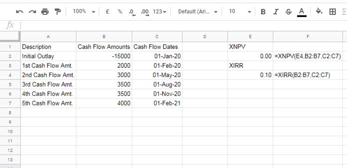
That’s all. Enjoy!