")
")


")


")

")
")
 in Excel & Google Sheets")


Today, I’ll show you how to use the SMALL function for both basic and advanced calculations in Google Sheets. This function finds the nth smallest element in a list you choose.
At first glance, the Google Sheets SMALL function seems simple. However, it can assist with lookup or offset operations by finding the nth occurrence. To achieve this, we will use a logical test with the IF and SEQUENCE functions.
We’ll explore this advanced tip after covering the syntax and basic formula examples of the SMALL function.
SMALL Function Syntax and Arguments
Syntax:
SMALL(data, n)
Arguments:
The SMALL function has two arguments:
data: This is the array or range that contains the dataset you want to evaluate.n: This specifies the rank, from smallest to largest, of the element you want to retrieve.
Basic Formula Examples
In a sequence from 1 to 10, setting ‘n’ to 3 will return 3, as it is the third smallest value in the dataset.
For example, use this formula to find the 3rd smallest value in column B:
=SMALL(B:B, 3)The SMALL formula returns a #NUM! error when:
- The range contains fewer than ‘n’ numbers
- The range is empty
- The range contains only text values.
What happens with multiple occurrences of numbers in the ‘data’ used with SMALL?
To understand this, try the following formula in your sheet. It will return 2 as the third smallest value in the provided array.
=SMALL({1, 2, 2, 3}, 3)You can specify multiple ‘n’ values within the SMALL function as an array. When doing so, remember to use the ARRAYFORMULA function. Here’s an example:
=ArrayFormula(SUM(SMALL(B1:B10, {1, 2, 3})))This formula calculates the sum of the first, second, and third smallest values in the range B1:B10.
SMALL Function to Locate the Nth Occurrence of a Text in Google Sheets
For example, in a sheet, I have fruit names in the range A2:A, such as Apple, Mango, Orange, etc. Some of the fruit names appear multiple times.
I want to find the relative position of the second occurrence of the item Mango. How do we find it?
| Apple |
| Mango |
| Orange |
| Mango |
| Strawberry |
| Grape |
| Mango |
| Blueberry |
| Pineapple |
| Watermelon |
| Cherry |
| Pineapple |
| Pineapple |
There are many methods. Here is one approach using the SMALL function in combination with IF and SEQUENCE.
The following formula will return 4, which is the relative position of the second occurrence of Mango in the range A2:A.
=ArrayFormula(SMALL(IF(A2:A="Mango", SEQUENCE(ROWS(A2:A)),), 2))You can use this function in combination with the INDEX function to offset that many rows in another column and get the corresponding value. First, we will see the explanation of the above formula.
Formula Breakdown
SEQUENCE(ROWS(A2:A)): Returns a sequence of numbers from 1 to the number of rows in the range A2:A.IF(A2:A="Mango", …, ): Returns an empty sequence number wherever A2:A doesn’t contain the fruit name Mango.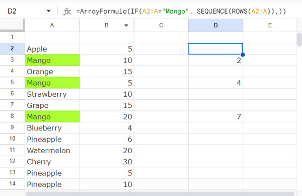
SMALL(…, 2)– Returns the second smallest value in the above data.
SMALL With INDEX to OFFSET Rows
Now let’s see how to use the relative position to offset rows in B2:B using the INDEX function.
Syntax:
INDEX(reference, [row], [column])Formula:
=INDEX(B2:B, SMALL(IF(A2:A="Mango", SEQUENCE(ROWS(A2:A)),), 2))Where:
reference:B2:Brow:SMALL(IF(A2:A="Mango", SEQUENCE(ROWS(A2:A)),), 2)
Note: I’ve omitted ARRAYFORMULA within INDEX as it’s not necessary here.
This INDEX and SMALL combo formula will return the value in B2:B corresponding to the 4th row in the range, which matches the second occurrence of “Mango” in column A.