The MODE function is a statistical function in Google Sheets that operates on numbers and dates, not on text values.
In statistics, the term ‘mode’ refers to the most frequently occurring value in a dataset.
However, the MODE function has a limitation: in a dataset in Google Sheets, there can be one mode, two modes, or more. In the case of multiple modes, the function will return the first mode encountered in the dataset.
We will explore this further in the example section below. But first, let’s review the syntax of the function.
MODE Function: Syntax and Arguments
Syntax:
MODE(value1, [value2, …])Arguments:
value1: The first value or range to consider.value2: (Optional) Additional values or ranges to consider.
If you specify ranges in value1 and value2, they can be of different sizes. Unlike other functions, this won’t result in a “Mismatched range sizes” error.
Now, let’s explore examples of using the MODE function in Google Sheets.
MODE Function with Numeric Ranges in Google Sheets
In the following example, I have the numbers 100, 100, 25, 25, and 100 in the range B5:B9. The most frequently occurring number among these numbers is 100.
You can use the following MODE formula to find it:
=MODE(B5:B9)
The above dataset is Unimodal as it has only one mode.
Let’s consider the following array which has two modes (Bimodal):
{5, 5, 6, 6, 6, 6, 6, 5, 5}The following MODE formula will return 5, which is one of the modes with the same highest frequency, as it appears first in the array.
=MODE({5, 5, 6, 6, 6, 6, 6, 5, 5})The same applies to a dataset that has more than two modes (Multimodal).
If no value occurs more than once (No Mode), the formula will return #N/A.
Additional Tips
If you have data in multiple ranges, you can use them within the MODE function either individually as value1, value2, and so on, or combined.
For example:
=MODE(A1:A10, B1:B10)
=MODE(A1:B10)
Additionally, you can use ranges with different sizes like =MODE(A1:A10, E5:E100).
MODE Function with Date Ranges in Google Sheets
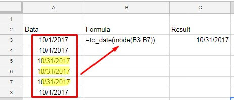
The MODE function in Google Sheets can return the mode of dates. The usage is the same as with numbers, with the addition of formatting.
The result of MODE will be a date value. You should format it back to a date using either the TO_DATE function or by formatting the result cell to a date.
Example:
=TO_DATE(MODE(B3:B7))If you prefer not to use the TO_DATE function, format the result to a date by clicking Format > Number > Date.

Identifying the Most Frequent Months or Years in a Date Column
From a date column, you can find the most frequently occurring month, year, or month and year. For that, you may require some other functions such as DATEVALUE, EOMONTH, IFERROR, and TEXT with the MODE function.
The formula should be entered as an array formula due to the aforementioned use of non-array functions with the MODE function.
The sample data is in B2:B, which consists of dates or timestamps.
You can use the following MODE formulas to find the mode of month, year, and month and year.
Mode of Month:
=ArrayFormula(MODE(IFERROR(MONTH(DATEVALUE(B2:B)))))The DATEVALUE function converts the dates to date values and returns errors in blank cells. Then MONTH converts those dates to month numbers. If we don’t first use DATEVALUE, MONTH will return 12 in blank cells and that will affect the MODE.
IFERROR removes errors, and MODE returns the mode of month numbers.
Mode of Year:
=ArrayFormula(MODE(IFERROR(YEAR(DATEVALUE(B2:B)))))This is similar to the above formula. Here we used the YEAR function instead of MONTH. The YEAR function converts a blank cell to 1899. So here also the use of DATEVALUE justifies.
Mode of Month and Year:
=ArrayFormula(TEXT(MODE(IFERROR(EOMONTH(DATEVALUE(B2:B), 0))), "MMM-YY"))The DATEVALUE function converts the dates to date values and returns errors in blank cells. Then EOMONTH converts those dates to end-of-the-month dates. If we don’t first use DATEVALUE, EOMONTH will return 31/12/1899 in blank cells and that will affect the MODE.
IFERROR removes errors, and MODE returns the mode of end-of-the-month dates. The TEXT function returns the month name.


