")
")


")


")

")
")
 in Excel & Google Sheets")


Not all Google Sheets functions have optional arguments, but many do. Let’s explore how to skip optional arguments in such functions in Google Sheets.
When checking a function’s syntax, you can identify optional parameters if they are enclosed in square brackets.
Skipping an optional parameter depends on its position in the syntax and is also function-specific.
There are hundreds of functions in Google Sheets, so it’s not feasible to cover all of them. Instead, this guide provides a general understanding of skipping optional parameters in Google Sheets functions.
I’ve selected a few functions to illustrate this concept.
Optional Arguments at the End or Middle of a Function Syntax
If an optional parameter appears at the end of a function’s syntax, you can usually skip it. However, be aware of the outcome.
When you omit the last optional argument, the function assigns its default value. So, understanding the default value is essential.
If you want to exclude multiple optional arguments, most functions will assign default values, but there are exceptions.
Skipping All Optional Arguments in a Function in Google Sheets
Example #1 – Single Parameter
Consider the VLOOKUP function. Its syntax is:
VLOOKUP(search_key, range, index, [is_sorted])The is_sorted parameter is optional because it’s enclosed in square brackets. Its default value is TRUE (1), meaning the data is sorted. If the data is not sorted, specify FALSE (0).
Example:
Assume the following dataset in A2:B5 (excluding headers):
| Category | Total Order |
|---|---|
| SUV | 5 |
| Compact SUV | 6 |
| Sedan | 5 |
| Hatchback | 4 |
The search key is “sedan”, and the index number (result column position) is 2.
=VLOOKUP("sedan", A2:B5, 2, FALSE)Here, the is_sorted argument is explicitly set to FALSE because the data is unsorted.
If the table is sorted:
| Category | Total Order |
| Compact SUV | 6 |
| Hatchback | 4 |
| Sedan | 5 |
| SUV | 5 |
Then, the last argument can be omitted:
=VLOOKUP("sedan", A2:B5, 2)Alternatively, if the data is unsorted, you can use:
=VLOOKUP("sedan", SORT(A1:B5), 2)Understanding the default values of optional arguments helps you decide when to exclude them.
Example #2 – Multiple Parameters
Some functions allow skipping all optional arguments. Consider GROWTH and TREND:
GROWTH(known_data_y, [known_data_x], [new_data_x], [b])
TREND(known_data_y, [known_data_x], [new_data_x], [b])
To skip all optional arguments, exclude them entirely:
=GROWTH(A2:A7)
=TREND(A2:A7)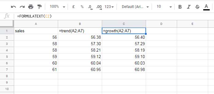
However, skipping only some optional arguments is different.
Skipping Some Optional Parameters in Google Sheets
Replacing known_data_x and new_data_x with Dummy Values
The b parameter in GROWTH and TREND stands for the curve fit. By default, it’s TRUE (1).
If you want to use b = FALSE (0) but skip known_data_x and new_data_x, generate a sequence of numbers for these arguments:
=SEQUENCE(6,1)Use this sequence in the formula:
=GROWTH(A2:A7, SEQUENCE(6,1), SEQUENCE(6,1), TRUE)
=TREND(A2:A7, SEQUENCE(6,1), SEQUENCE(6,1), TRUE)
Changing TRUE to FALSE modifies the behavior, allowing you to exclude middle arguments effectively.
Using Commas to Skip Optional Parameters in Financial Functions
Some functions, especially financial ones, allow skipping optional arguments by placing a comma.
Example: PMT function
PMT(rate, number_of_periods, present_value, [future_value], [end_or_beginning])Inputs (C2:C6):
- rate = 1%
- number_of_periods = 12
- present_value = 30,000
- future_value = (skipped)
- end_or_beginning = 1
Formula:
=PMT(C2, C3, C4,, C6)The double comma (,,) skips the optional future_value parameter.
Conclusion
In some functions, you can even skip required arguments. For example, in IF:
IF(logical_expression, value_if_true, value_if_false)Example:
=IF(A1="",,A1*5.5)This formula omits value_if_true, allowing for more flexible logic.
Although these arguments are not enclosed in square brackets, one of the last two parameters is technically optional—you can choose which one to omit.
To summarize, understanding the default values of optional arguments in Google Sheets functions enables you to determine when and how to skip them.
That’s all! Enjoy!