You can approach finding the lowest-priced items from two angles: using a unique list or a list with multiple occurrences of items.

If you have a unique list, the approach will involve finding the minimum value and then filtering all the items that match that value. This method is useful for identifying vendors who quoted the lowest price.

In cases with multiple occurrences, we will find the lowest price for each item and display all those items. This approach is beneficial when you want to filter vendors who quoted the lowest prices for multiple items.

To illustrate these methods, let’s look at some examples.

Find All Lowest-Priced Items in a Unique List

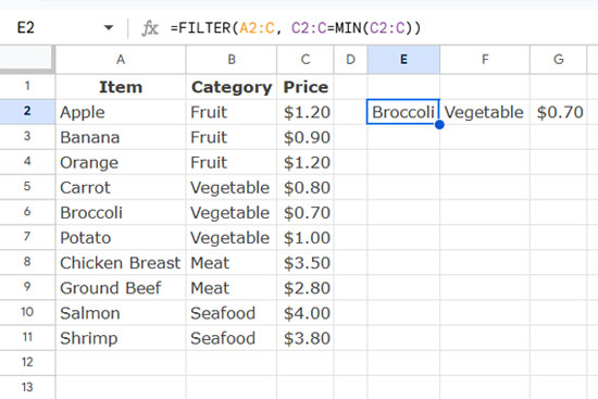
In this example, we have a table with Item, Category, and Price in columns A, B, and C, respectively, with A1:C1 reserved for headers.

The following FILTER formula will return the lowest-priced item from this list:

=FILTER(A2:C, C2:C=MIN(C2:C))

The FILTER function filters the range A2:C based on a specified condition. In this case, the condition is C2:C=MIN(C2:C), which means it returns rows where the price matches the minimum value in the Price column (C2:C).

This approach will return all items that share the lowest price in the list.

If you view this from the perspective of vendors and their quoted prices for a particular item, consider column A filled with the same item, column B with vendor names, and column C with their respective quoted prices.

Extract the Lowest-Priced Items by Category

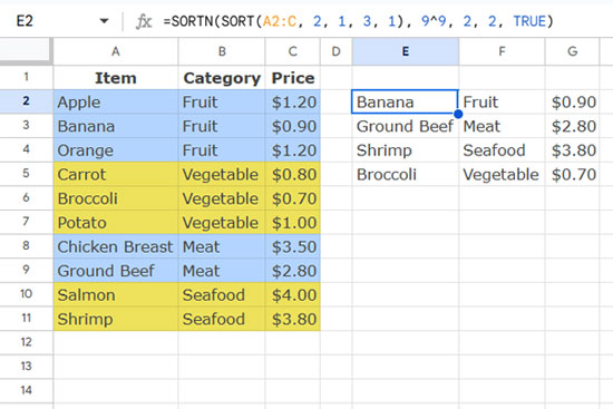
Sometimes, you may want to find the lowest-priced items from each category. In the previous example, consider the Category column (B).

In this scenario, we will use a combination of the SORT and SORTN functions.

The SORT function will sort the table by category and then by price in ascending order, so the lowest-priced items in each category will be at the top.

Then we’ll use the SORTN function to return the unique categories along with their lowest-priced items:

=SORTN(SORT(A2:C, 2, 1, 3, 1), 9^9, 2, 2, TRUE)

If you view this from the perspective of vendors and their quoted prices for multiple items, consider column A filled with unique vendor names, column B filled with items, and column C filled with their respective quoted prices.

Formula Breakdown

• Syntax: SORTN(range, [n], [display_ties_mode], [sort_column], [is_ascending], [sort_column2, …], [is_ascending2, …])

Where:

• range: SORT(A2:C, 2, 1, 3, 1) sorts the data first by category (column B) and then by price (column C) in ascending order, placing the lowest-priced items at the top of each category.
• n: 9^9 is an arbitrarily large number that specifies the maximum number of rows to return, as we cannot predict how many unique categories there will be.
• display_ties_mode: 2 indicates that duplicates should be removed.
• sort_column: 2 indicates that the removal of duplicates will occur based on the second column (the category).
• is_ascending: TRUE specifies that the output should be sorted in ascending order.

This approach may pose a challenge if there are multiple items with the same lowest price within the same category. The SORTN function cannot retrieve these, as it removes duplicates by category.

Handling Multiple Lowest-Priced Items in the Same Category

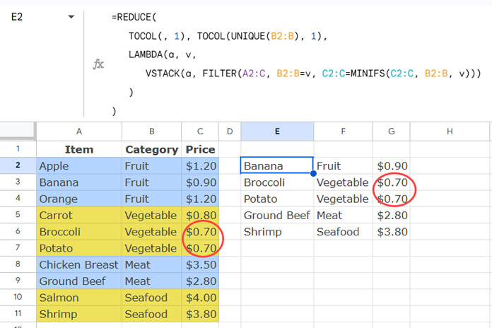
The lowest-priced item in the vegetable category is “Broccoli,” priced at $0.70. Let’s modify the price of “Potato” in the vegetable category to $0.70, down from $1.00.

The previous formula will only return one lowest-priced item from each category.

In this case, we can use a more complex formula that involves the REDUCE LAMBDA function. Here’s the formula:

=REDUCE(
   TOCOL(, 1), TOCOL(UNIQUE(B2:B), 1), 
   LAMBDA(a, v, 
      VSTACK(a, FILTER(A2:C, B2:B=v, C2:C=MINIFS(C2:C, B2:B, v)))
   )
)

Formula Explanation

LAMBDA functions can be tricky to explain, but understanding the core concepts can help you grasp their functionality.

Syntax: REDUCE(initial_value, array_or_range, lambda)

• TOCOL(UNIQUE(B2:B), 1): This returns the unique categories from column B and removes any empty cells. This is the array (array_or_range) used in the REDUCE function.
• REDUCE function: This function uses an accumulator to store intermediate values during the calculation. The initial value is TOCOL(,1) (initial_value), which represents an empty cell.
• The REDUCE function applies a LAMBDA to each value in the array (array_or_range), processing one row at a time.

Here’s a detailed look at the LAMBDA function:

• LAMBDA(a, v, VSTACK(a, FILTER(A2:C, B2:B=v, C2:C=MINIFS(C2:C, B2:B, v)))): This filters the range A2:C based on two conditions:
  • B2:B=v (where ‘v’ is an element from the unique categories array).
  • C2:C=MINIFS(C2:C, B2:B, v) which finds the minimum price for that specific category.

Essentially, the FILTER function extracts the rows that contain the minimum price for each category, and the REDUCE function iteratively applies this to each unique category.

The accumulator defined as ‘a’ is vertically stacked, resulting in a final output that includes all items with the lowest prices from each category.

Resources

• Filter Min or Max Value in Each Group in Google Sheets
• How to Highlight the Min Value in Each Group in Google Sheets