


")


")

")
")
 in Excel & Google Sheets")


Filtering duplicates is often necessary when editing or removing data in Google Sheets. While the built-in command (Data > Data Cleanup > Remove duplicates) is convenient for removing duplicates, it doesn’t allow you to view them beforehand. Filtering duplicates offers this advantage.
Once you’ve filtered duplicates, you can select the visible rows, right-click, and delete them. Alternatively, you can apply a fill color to make them stand out.
Before You Start
The term “duplicate” can be categorized into three scenarios:
- Column-Based Duplicates: Duplicate records are identified when the same value appears multiple times within a specific column.
- Custom/Selected Column-Based Duplicates: Duplicate records are identified when selected columns have the same values in each row, regardless of other data in the row.
- Row-Based Duplicates: Duplicate records are identified when an entire row (all columns) is repeated multiple times.
You’ll need different formulas for each scenario to filter duplicates. Let’s dive into examples for each case.
How to Filter Column-Based Duplicates in Google Sheets
Imagine you have a list of names in column A with “Name” in cell A1:
| Name |
| Saket |
| Saket |
| Saket |
| Elizabeth |
| Elizabeth |
| Ben |
| Emily |
To filter duplicates in column A:
- Select column B (a blank column).
- Go to Data > Create a Filter.
- Click the filter icon in B1 and choose Filter by Condition > Custom formula is.
- Enter the formula:
=COUNTIF($A$2:A2, A2) > 1 - Click Done.
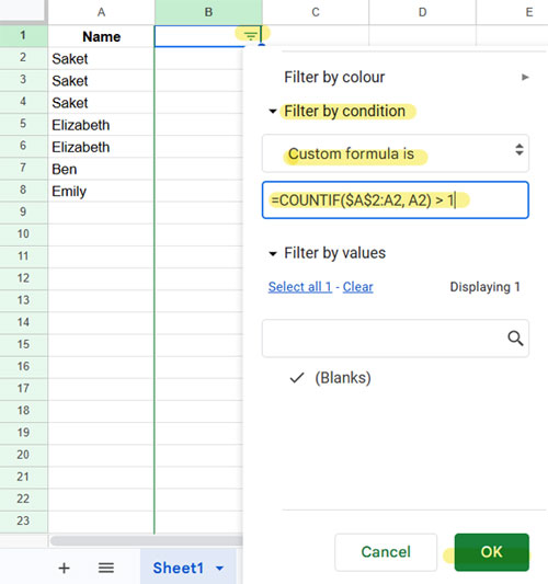
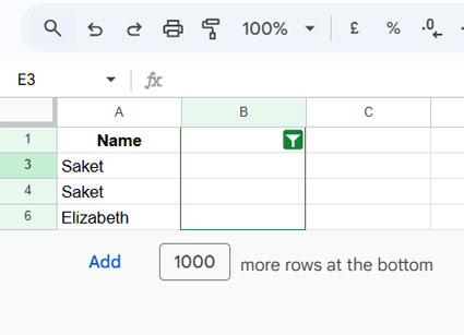
This formula counts the occurrences of values in column A up to the current row.
$A$2is the fixed start of the range.A2dynamically adjusts as the formula processes each row.
The formula returns TRUE wherever the count exceeds 1, effectively filtering duplicates.
How to Filter Custom/Selected Column-Based Duplicates in Google Sheets
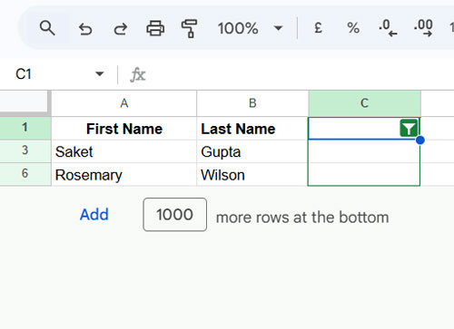
Suppose you have a dataset like this in A1:B:
| First Name | Last Name |
| Saket | Gupta |
| Saket | Gupta |
| Saket | Patel |
| Rosemary | Wilson |
| Rosemary | Wilson |
| Ethan | Johnson |
Here, a duplicate occurs when the same first name and last name appear more than once in the rows.
To filter these duplicates:
- Select column C (a blank column).
- Go to Data > Create a Filter.
- Use the following custom formula:
=COUNTIFS($A$2:A2, A2, $B$2:B2, B2) > 1This formula counts the occurrences of first and last names in columns A and B up to the current row, and returns TRUE if the count is greater than 1. The formula adjusts dynamically in the filtered range because we used a fixed start and relative end range, along with relative criteria.
How to Filter Row-Based Duplicates in Google Sheets
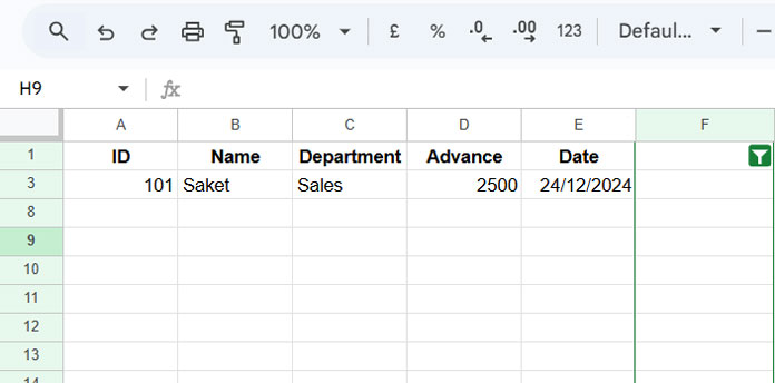
In the following dataset in A1:E, let’s filter rows where all columns—ID, Name, Department, Advance, and Date—are identical.
| ID | Name | Department | Advance | Date |
| 101 | Saket | Sales | 2500 | 24/12/2024 |
| 101 | Saket | Sales | 2500 | 24/12/2024 |
| 101 | Saket | Sales | 2500 | 21/01/2025 |
| 102 | Elizabeth | Marketing | 1000 | 24/12/2024 |
| 103 | Elizabeth | HR | 1000 | 24/12/2024 |
To filter row-based duplicates, use the following formula:
=COUNTIFS($A$2:A2, A2, $B$2:B2, B2, $C$2:C2, C2, $D$2:D2, D2, $E$2:E2, E2) > 1This approach is similar to the selected column-based method from the second example above. While it works, specifying many columns can be tedious. Here’s a dynamic alternative:
=COUNTIF(TRANSPOSE(QUERY(TRANSPOSE($A$2:E2),,9^9)), TRANSPOSE(QUERY(TRANSPOSE(A2:E2),,9^9)))>1This formula dynamically evaluates the entire range, eliminating the need to list each column individually.
Deleting or Highlighting Filtered Rows
After filtering duplicates, you can take one of the following actions:
- Delete Filtered Rows:
- Select the visible rows (excluding the header).
- Right-click and choose Delete selected rows.
- Highlight Filtered Rows:
- Select the visible rows.
- Click the paint bucket icon in the toolbar to apply a fill color.
Resources
- Find and Eliminate Duplicates Using QUERY in Google Sheets
- Removing Duplicates In Google Sheets: Built-In Tool & Formulas
- How to Insert Duplicate Rows in Google Sheets
- How to Prevent Duplicates in Google Sheets
- Combine Duplicate Rows in Google Sheets
- Merging Duplicate Rows Using Array Formulas in Google Sheets