Why add leading zeros in Google Sheets? The answer is simple: to make all the numbers in a column equal in length or visually identical.
There are two methods to add leading zeros, depending on your needs:
- Custom Number Formatting: Add leading zeros to the existing range without altering the data type.
- Using a Formula: Add leading zeros using a formula without affecting the source data. The result will be in a new range. This method has two options:
- QUERY Formula: Maintains the data type as numbers.
- TEXT Formula: Converts the numbers to text.
Adding Leading Zeros with Custom Number Formatting in Google Sheets
This method retains the number data type.
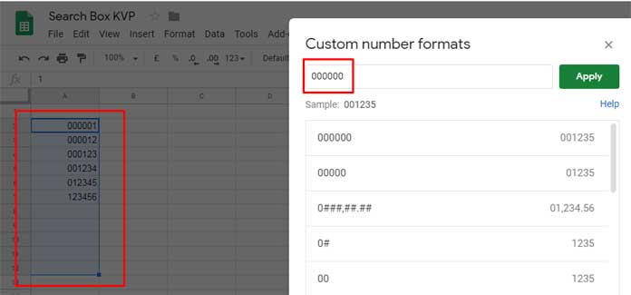
If you have numbers in a range and want to automatically apply leading zeros without changing the data type, follow these steps. This method ensures that the numbers remain as numbers, so calculations using those numbers won’t be affected.

- Select the range where you want to add leading zeros in your Google Sheets file.
- Click Format > Number > Custom number format.
- Decide the maximum number of digits you may enter in the selected cells. For example, if you plan to enter numbers ranging from 1 to 6 digits, enter six zeros in the custom field.
- Click the Apply button.
This will add leading zeros without changing the data type in the selected range. If you have decimal numbers, the decimal part might become hidden.
To make the decimal part visible, click the Increase Decimal Places button on the toolbar. The numbers will remain uniform in length.
Note: To remove the leading zeros, select the range and click Format > Number > Automatic.
Adding Leading Zeros Using Formulas in Google Sheets
When using a formula to add leading zeros, keep in mind that the output will be text or number formatted depending on the formula used.
For example, to make the numbers in the range A2:A10 equal in length, use the following TEXT array formula in cell B2:
=ArrayFormula(IF(A2:A10="", ,TEXT(A2:A10, "000000"))The output of this formula will be text-formatted.
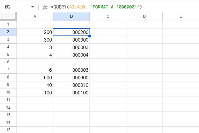
Another option is the QUERY formula:
=QUERY(A2:A10, "FORMAT A '000000'")This formula will also add leading zeros to the numbers in the range A2:A10. If you enter this formula in cell B2, you’ll see that the values in the range B2:B10 will be formatted as numbers, not text.

You can adjust the number of zeros according to the length you need.
If you want to display decimals as well, replace 000000 in both formulas with 000000.00.
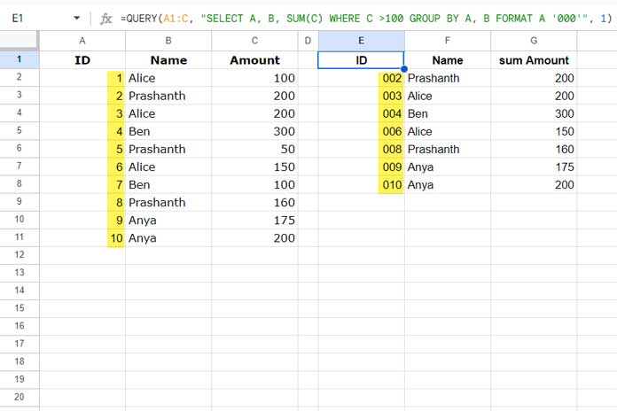
The QUERY function offers advanced data manipulation capabilities. For example, if you have employee data with ID, Name, and Advance Amount in columns A, B, and C respectively, the following QUERY formula will filter the data for employees whose advance amount is greater than 100 and add leading zeros to the ID column:
=QUERY(A1:C, "SELECT A, B, SUM(C) WHERE C >100 GROUP BY A, B FORMAT A '000'", 1)
Additional Tip
If you want to add leading zeros and don’t need to worry about specific digit length or formatting, simply start the number with an apostrophe.
For example, to enter 0001 in cell A1, type it as '0001.
Resources
- Formatting Date, Time, and Numbers in Google Sheets Query
- How to Concatenate a Number without Losing Its Format in Google Sheets
- How to Format Numbers as Fractions in Google Sheets
- Format Numbers as Currency Using Formulas in Google Sheets
- How to Sort Numbers Formatted as Text in Google Sheets (Formula Approach)
- Format Numbers To Millions and Thousands in Google Sheets
- Format a Date Without Converting it Into a Text – Google Sheets


