Data validation is a powerful feature in Google Sheets that helps maintain data quality by preventing incorrect or duplicate entries. This tutorial demonstrates how to use Data validation to stop duplicates in Google Sheets using custom formulas.
Why Use Data Validation to Prevent Duplicates?
Data validation ensures data accuracy by enforcing specific rules during data entry. While Google Sheets has many built-in rules, it lacks a default option to prevent duplicate entries. By using a custom formula, you can efficiently block duplicates across a range, ensuring clean and reliable data.
Features of the Custom Formula Rule
Here are the key features of my data validation rules that help prevent duplicates in your sheet.
- Versatility: The formula can prevent duplicates in:
- Single or multiple columns
- A selected range
- An entire tab
- Supports Unique Combinations:
It can also prevent duplicate combinations of two columns, making it useful for datasets with dependent values like product IDs and items. - Set-and-Forget:
Once applied, the rule automatically prevents duplicates without requiring further adjustments. - Customizable Limit:
Depending on your requirements, you can allow duplicates up to a specified number of times. - Flexible Response:
Choose to either reject duplicates outright or flag them for review.
How to Prevent Duplicates in Google Sheets
Step-by-Step Guide to Applying Data Validation
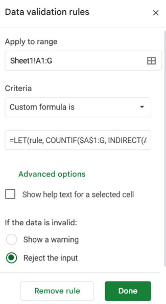
Follow these steps to prevent duplicates in the range A1:G using a custom formula:

Formula:
=LET(rule, COUNTIF($A$1:G, INDIRECT(ADDRESS(ROW(), COLUMN(),))), ISBETWEEN(rule, 1, 1))Steps:
- In your Google Sheet, select the range where you want to apply the rule (e.g.,
A1:G). - Go to Data > Data validation in the menu.
- Click the + Add rule button in the sidebar.
- Under Criteria, select Custom formula is and paste the formula.
- Under Advanced options, decide whether to:
- Show a warning: Flag duplicates for review.
- Reject the input: Block duplicates from being entered.
- Click Done to apply the rule.

In the above steps, we used the formula for the range A1:G. If your range is different, replace $A$1:G in the formula with the desired range, such as $C$1:C100.
How to Allow Duplicates a Limited Number of Times
If you need to allow duplicates up to n times, modify the formula accordingly.
Example: Allow Duplicates Twice
Formula:
=LET(rule, COUNTIF($A$1:G, INDIRECT(ADDRESS(ROW(),COLUMN(),))), ISBETWEEN(rule, 1, 2))As you can see, the change is minimal. I have simply replaced the third argument in the ISBETWEEN function from 1 to 2. This demonstrates that the third argument controls the value of n (the maximum number of allowed duplicates).
This formula permits duplicates to appear up to two times.
For a specific column (e.g., column A), update the range $A$1:G to $A$1:A.
Steps:
- Follow the same data validation steps as above.
- Use this modified formula instead.
Preventing Duplicate Combinations of Two Columns
Previously, we discussed rejecting duplicate values outright. In that context, a duplicate was defined as a single value appearing more than once, prompting it to be flagged or rejected.
But what if you want to prevent duplicate combinations across two columns?
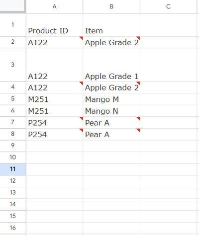
For instance, imagine you have data in columns A and B with headers in row 1 (e.g., A1:B1). Column A contains Product IDs, and column B contains Items. If the same Product ID and Item combination appear more than once, you might want to flag it or reject the input.
Here’s the rule to prevent duplicate combinations for the range A2:B, leaving the header row untouched:
=LET(rule, ArrayFormula(COUNTIFS($A$2:$A&"|"&$B$2:$B, $A2&"|"&$B2)), ISBETWEEN(rule, 1, 1))
Steps:
- Select the range where the rule should apply (e.g.,
A2:Bexcluding the header row). - Open Data validation and add a new rule.
- Paste the above formula into the Custom formula is field.
- Choose whether to flag or reject duplicate combinations.
- Click Done.
This ensures unique combinations of values across two columns.
Important Note: Copy-Pasting and Data Validation
Data validation works only during manual data entry or formula-driven changes. Copy-pasting bypasses validation, meaning duplicate entries can still be added this way.
Tips to Address This:
- Add a bold, highlighted note at the top of your sheet warning users about the limitations of copy-pasting.
- Regularly review your data for duplicates using the Remove Duplicates tool in Google Sheets.


Hi!
Just found this trying to prevent duplicates in a sheet, But I have unique data based on 2 cells in a row , “SET” and “ID”
Is there any way to prevents duplicate Combinations of the 2? As both will have duplicates individually (IE Set will have the Value GP1 Several times, And ID will have the value 3 several times) But The same combined Value should not be allowed (IE the Combination of GP1 3 can’t be duplicate)
I’ve updated the post to include a section that addresses your problem. I’ve also modified the earlier formulas for greater flexibility. I hope you check it out and leave your feedback below.
Hi, Prashanth,
I have an HTML form submitted to Google Sheets when it’s filled out.
But every time a new entry is created, it duplicates the entry in Google Sheets and sends two email notifications.
It should be one entry to Sheets and one email notification. Have you ever seen anything like this or possibly have a fix?
Hi, Chris,
Sorry! I’ve no idea about that.
It is possible to prevent duplicate values across all the sheets in a workbook instead of on just one sheet?
Hi, Aaran,
Right now, you can’t specify a workbook as a whole. But you can of course specify individual sheets in a workbook one by one.
This conditional formatting is an example:
How to Conditional Format Duplicates Across Sheet Tabs in Google Sheets.
Hi, I want
My Sheet1 C2:C get data validations and don’t make duplicates from another sheet range J1:J
Is that possible using data validation?
Hi, Guenahel,
I hope you can find an answer to your this data validation query in one of my earlier posts here – Reject a List of Items in Data Validation in Google Sheets.
Hi there. Is it possible to check for several ranges at the same time? Different sheets with similar information? If so, how do I do that? I can’t seem to “ctrl – Select” them all, nor comma it’s ranges.
Hi, Max,
I have conditional formatting to highlight duplicates across the tabs.
How to Conditional Format Duplicates Across Sheet Tabs in Google Sheets.
Are you looking for data validation to reject input depending on duplicates in multiple tabs?
If so, please elaborate on the problem.
Is it possible to check for a maximum number of occurrences as your formula allows AND the entered number to be less than a stated number?
For example, I want to allow a maximum number of duplicates to be 4 and the entered number to be between 1 and 20 (> 0 but < 21).
Hi, Tom,
Try this formula, please.
=and(existing formula,and(A1>0,A1<20))Best,
Does work if you copy and paste the data, rather than manually type it in.
If you fill the cells down, it won’t work either.
Hi, Leo,
That’s correct! The “reject input” may not have any effect. But the duplicates will get flagged anyhow.
The problem with data validation and conditional formatting are it get copied along with the values.
Thanks, it has worked. Now, will the formula apply to all data entered in column A? Again, how can I disable the main menu to allow the users just to enter data only without interfering with my settings?
Hi, Herbert,
It depends on the range that you have selected. I am talking about the “Cell range” in the data validation settings. You can refer my screenshot above where I have selected the range A1:G. For entire column A you can change that to A1:A.
I don’t know anything about disabling menu in Google Sheets. I suggest you to use the Protect Sheet feature that you can find under the Tools menu in Google Sheets. Only give access to the required cell range for editing. This probably prevents them from interfering with your settings.
Check this Google Sheets Documentation for more details.
https://support.google.com/docs/answer/1218656?co=GENIE.Platform%3DDesktop&hl=en