Horizontal Running Total in Google Sheets

A horizontal running total is the cumulative sum of values across a row. It adds each number to the sum of all previous numbers in the same row.

Example:

Assume we are selling white pebbles, and we’ve recorded the sales data for the past week in the range B3:G3:

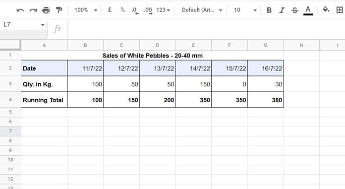
We want the output in B4:G4 to be:

100, 150, 200, 350, 350, 380

Horizontal Running Total in Google Sheets – Easiest Formulas

✅ Non-Array Formula

=SUM($B$3:B3)

Enter this formula in cell B4 and drag it across to the right. The first cell reference stays fixed (absolute) while the second adjusts (relative) as follows:

Cell	Formula
B4	=SUM($B$3:B3)
C4	=SUM($B$3:C3)
D4	=SUM($B$3:D3)
E4	=SUM($B$3:E3)
F4	=SUM($B$3:F3)
G4	=SUM($B$3:G3)

✅ Array Formula Using SUMIF

=ArrayFormula(
   SUMIF(
      COLUMN(B3:G3), 
      "<=" & COLUMN(B3:G3), 
      B3:G3
   )
)

Clear any content in B4:G4 and enter the formula in B4.

This formula will return the horizontal running total for the sales quantity of white pebbles.

If row 2 contains dates, you can now easily read the cumulative total of pebbles sold up to each date from row 4.

Explanation of the Array Formula

Let’s break it down using the SUMIF syntax:

SUMIF(range, criterion, [sum_range])

range – COLUMN(B3:G3)
criterion – "<=" & COLUMN(B3:G3)
sum_range – B3:G3

This tells Google Sheets to sum the values in B3:G3 up to each column.

Example Evaluation (in C4):

COLUMN(B3:G3) = {2, 3, 4, 5, 6, 7}

Criterion for C4: <= 3

Evaluation: {2<=3, 3<=3, 4<=3, 5<=3, 6<=3, 7<=3} → {TRUE, TRUE, FALSE, FALSE, FALSE, FALSE}

Only the first two values in B3:G3 will be included in the sum.

Other Horizontal Running Total Formulas for Advanced Users

You may skip these formulas unless you’re comfortable with more advanced techniques. They can be useful in some scenarios but are less intuitive than the previous examples.

Non-Array Formula:

=N(A4) + B3

Place this formula in B4 and drag it across. It accumulates the values by adding the new value to the previous total.

MMULT Formula (Array):

=ArrayFormula(
   MMULT(
      N(B3:G3), 
      IF(COLUMN(B3:G3) >= TRANSPOSE(COLUMN(B3:G3)), 1, 0)
   )
)

This formula uses matrix multiplication to simulate a running total across a row. It’s fast but can be difficult to customize or debug.

DSUM Formula (Array):

=ArrayFormula(
   DSUM(
      {B3:G3; TRANSPOSE(IF(SEQUENCE(6,6)^0 + SEQUENCE(6,1,COLUMN(B3)-1) >= COLUMN(B3:G3), B3:G3))}, 
      SEQUENCE(1,6), 
      {IF(,,); IF(,,)}
   )
)

A more complex option using DSUM and structured criteria. Useful in niche scenarios but not recommended for everyday use.

✅ SCAN Formula (LAMBDA Function):

=SCAN(0, B3:G3, LAMBDA(a, v, a + v))

The SCAN function offers a clean and modern way to calculate running totals using LAMBDA. Ideal for dynamic arrays and readable logic.

How to Calculate a Horizontal Running Total in Google Sheets