How to Properly Concatenate Start and End Times in Google Sheets

Recently, I helped one of my readers concatenate a start time with an end time in his preferred format in Google Sheets.

His preferred approach was to combine a 24-hour start and end time, format it to a 12-hour format, and retain the AM/PM notation in the output.

This process also involves removing unwanted substrings—such as duplicate “AM” or “PM” notations—which I will explain later.

In this tutorial, I will show you how to properly concatenate start and end times in Google Sheets while ensuring the correct formatting.

Concatenating Two Time Cells in Google Sheets and Formatting Issues

There’s an important time formatting consideration when concatenating time values.

Normally, when you concatenate a start and end time using the ampersand (&), the output loses its time formatting.

Consider the following example:

Start	End
10:00:25	21:25:00

Using a basic formula like:

=A2&" "&B2

Result: 0.416956018518519 0.892361111111111

Frustrating, right?

Using JOIN or TEXTJOIN produces a more readable result:

=JOIN(" - ", A2:B2)
=TEXTJOIN(" - ", TRUE, A2:B2)

Result: 10:00:25 - 21:25:00

However, I want the result to be formatted like this:

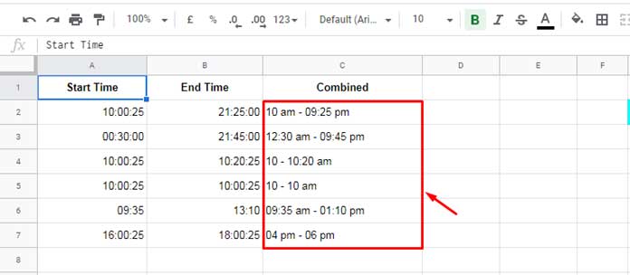
Expected Output: 10 am - 09:25 pm

I also want to:

☑ Remove seconds.
☑ Remove minutes if they are 00.
☑ Include AM/PM notation.
☑ Avoid repeating “AM” if both times fall in the morning.

If that sounds confusing, check out rows 4 and 5 in the example below.

Properly Concatenating Start Time with End Time in Google Sheets

Concatenate Start and End Times in Google Sheets – The Right Way

To properly concatenate start and end times in Google Sheets, we can use the TEXT function.

Let’s see how we can use TEXT with JOIN and & to format the output correctly.

Using TEXT and Ampersand (`&`)

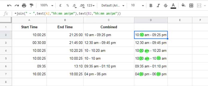
=TEXT(A2, "hh:mm am/pm")&" - "&TEXT(B2, "hh:mm am/pm")

Using TEXT and JOIN

=JOIN(" - ", TEXT(A2, "hh:mm am/pm"), TEXT(B2, "hh:mm am/pm"))

If applied in cell D2, you can drag the formula down to apply it to other rows.

Combining Two Time Cells the Normal Way in Google Sheets

Array Formula for Automatic Expansion

Instead of manually copying the formula, we can use an array formula to handle the entire column automatically:

=ArrayFormula(IF(A2:A="", "", TEXT(A2:A, "hh:mm am/pm") & " - " & TEXT(B2:B, "hh:mm am/pm")))

☑ Bonus Tip: The ampersand method works with array formulas, whereas JOIN requires MAP and LAMBDA.

If you’re curious, here’s how to use MAP and LAMBDA:

=MAP(A2:A, B2:B, LAMBDA(start, end, IF(start="", "", JOIN(" - ", TEXT(start, "hh:mm am/pm"), TEXT(end, "hh:mm am/pm")))))

The output in Column D is functional, but Column C has the ideal formatting. Let’s refine it further.

Removing Extra Strings After Concatenating Start and End Times in Google Sheets

Let’s refine the formatting further by:

☑ Removing :00 minutes when they exist.
☑ Avoiding duplicate AM/PM markers.

We will apply the following refinements step by step:

1. Basic Concatenation

Assume the start time is 10:00:25, and the end time is 10:20:25.

=TEXT(A2, "hh:mm am/pm") & " - " & TEXT(B2, "hh:mm am/pm")

Output: 10:00 am - 10:20 am

2. Remove `:00` from Minutes

Use REGEXREPLACE to eliminate unnecessary :00 values:

=TRIM(REGEXREPLACE(TEXT(A2, "hh:mm am/pm") & " - " & TEXT(B2, "hh:mm am/pm"), ":00", " "))

Output: 10 am - 10:20 am

3. Avoid Repeating “AM” or “PM”

Use REGEXREPLACE to remove redundant “AM” when both times are in the same period (i.e., the first half of the day):

=TRIM(REGEXREPLACE(REGEXREPLACE(TEXT(A2, "hh:mm am/pm") & " - " & TEXT(B2, "hh:mm am/pm"), ":00", " "), "^(\d+.*) am - (\d+.*) am$", "$1 - $2 am"))

Output: 10 - 10:20 am

4. Handle Empty Cells

If a cell is empty, the formula treats it as 00:00. To prevent this, wrap it in an IF statement:

=IF(A2="", "", TRIM(REGEXREPLACE(REGEXREPLACE(TEXT(A2, "hh:mm am/pm") & " - " & TEXT(B2, "hh:mm am/pm"), ":00", " "), "^(\d+.*) am - (\d+.*) am$", "$1 - $2 am")))

5. Apply to an Entire Column (Array Formula)

To apply this formula across a range, modify it as an array formula:

=ArrayFormula(IF(A2:A="", "", TRIM(REGEXREPLACE(REGEXREPLACE(TEXT(A2:A, "hh:mm am/pm") & " - " & TEXT(B2:B, "hh:mm am/pm"), ":00", " "), "^(\d+.*) am - (\d+.*) am$", "$1 - $2 am"))))

Now, the formula properly concatenates start and end times in Google Sheets while ensuring the correct formatting.

Sample Sheet