You can use a combination formula with WORKDAY.INTL as the key function to highlight the next N working days from a specific date in Google Sheets.

This formula requires you to specify:

1. The number of business days to highlight.
2. The weekends.
3. Any specific holidays to exclude.

These details will be incorporated into the formula, as explained below.

How Highlighting Next N Working Days Is Useful

Sometimes, you may need to commit to clients or stakeholders that you’ll complete tasks within the next 3, 7, or 10 working days from a specific date.

In such cases, you might want to highlight rows in your dataset where the task dates fall within the next N working days. Working days exclude weekends and holidays, making this functionality especially useful for accurate scheduling.

Example: Highlighting Next N Working Days

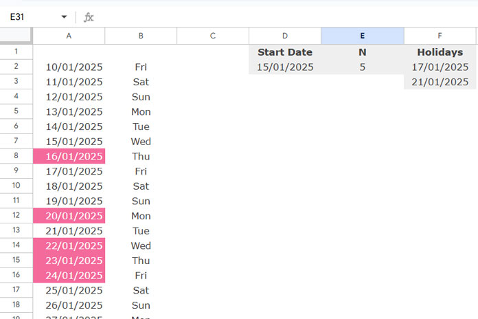
Assume the list of dates is in column A2:A.

1. Enter the specific start date in D2. This could be =TODAY() or any other date.
2. In E2, input the number of business days to highlight (e.g., 5).
3. Use F2:F to specify holidays to exclude from the highlighting.

Now, use the following custom formula in conditional formatting:

=AND(
   ISBETWEEN(
      A2, 
      WORKDAY.INTL($D$2, 1, "0000011", TOCOL($F$2:$F, 1)), 
      WORKDAY.INTL($D$2, $E$2, "0000011", TOCOL($F$2:$F, 1))
   ), 
   NOT(ISNUMBER(XMATCH(WEEKDAY(A2, 2), {6; 7}))),
   NOT(ISNUMBER(XMATCH(A2, TOCOL($F$2:$F, 1))))
)

This formula highlights the next 5 business days from the date in D2, excluding the holidays in F2:F. Here, “0000011” defines Saturday and Sunday as weekends.

Applying the Rule

• Select the range A2:A (the dates to be highlighted).
• Go to Format > Conditional formatting.
• Under Format rules, choose Custom formula is and paste the formula above.
• Select your preferred formatting style and click Done.

Now, the specified range will highlight the next N working days.

Customizing Weekends in the Formula

The formula uses a string to specify weekends within the WORKDAY.INTL function. The string contains seven characters where 0 represents a workday and 1 represents a weekend. For example:

• "0000011": Saturday and Sunday as weekends.
• "0000110": Friday and Saturday as weekends.

If you change the weekend string, remember to update:

1. Both occurrences of WORKDAY.INTL in the formula.
2. The array constants {6; 7} for the weekend days. For example, if your weekends are Friday and Saturday, replace it with {5; 6}.

Here’s the updated formula for Friday and Saturday weekends:

=AND(
   ISBETWEEN(
      A2, 
      WORKDAY.INTL($D$2, 1, "0000110", TOCOL($F$2:$F, 1)), 
      WORKDAY.INTL($D$2, $E$2, "0000110", TOCOL($F$2:$F, 1))
   ), 
   NOT(ISNUMBER(XMATCH(WEEKDAY(A2, 2), {5; 6}))),
   NOT(ISNUMBER(XMATCH(A2, TOCOL($F$2:$F, 1))))
)

How the Formula Works

Logical Expression 1:

ISBETWEEN(A2, next_n_start, next_n_end)

• WORKDAY.INTL($D$2, 1, "0000011", TOCOL($F$2:$F, 1)): Calculates the start date of the next N working days.
• WORKDAY.INTL($D$2, $E$2, "0000011", TOCOL($F$2:$F, 1)): Calculates the end date of the next N working days.
• ISBETWEEN checks if the date in A2 falls within this range.

Logical Expression 2:

NOT(ISNUMBER(XMATCH(WEEKDAY(A2, 2), {6; 7})))

Returns TRUE if the date in A2 is not a weekend.

Logical Expression 3:

NOT(ISNUMBER(XMATCH(A2, TOCOL($F$2:$F, 1))))

Returns TRUE if the date in A2 is not a holiday.

If all conditions are TRUE, the formula highlights the cell.

Resources

• Highlight Duplicate Values Based on Occurrence Days in Google Sheets
• Highlighting Today and N Cells Below in Google Sheets Calendar
• Highlight Upcoming Birthdays in Google Sheets
• Finding the Last 7 Working Days in Google Sheets (Array Formula)
• How to Find the Last Working Day of a Year in Google Sheets
• Find Number of Working and Non-Working Days in Google Sheets
• How to Find the Last Business Day of a Month in Excel