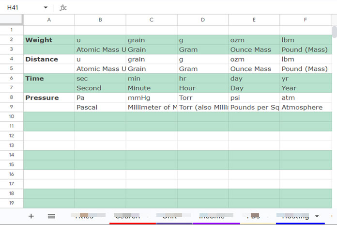
To highlight every alternate set of rows, or pairs of rows, in Google Sheets, you can use custom conditional formatting rules. This is especially useful when you have linked data across multiple rows.
For example, if you have 4 categories such as Weight, Distance, Time, and Pressure, with each category spanning two rows—one for units of measurement and the other for unit descriptions—you can apply a rule to highlight each pair of rows.
By using a custom rule, you can highlight each set of alternate rows, and this rule can be easily modified to highlight every n set of alternate rows.
Example: Highlighting Every 2 Sets of Alternate Rows
Here are the steps to follow:
- Select the range. For this example, let’s highlight the range A2:Z100 (but this can be any range).
- Click Format > Conditional formatting to open the sidebar panel.
- Under Format Rules, select Custom Formula is.
- Insert the following formula into the field:
=ISODD(ROUNDUP(ROW($A1)/2)). - Choose a highlighting style under Formatting Style.
- Click Done.
This will highlight every set of two alternate rows in the selected range.

As you can see, the chosen highlighting style applies to the first two rows, skips the next two rows, and then highlights the fifth and sixth rows, and so on.
If you want the highlighting to start from the third and fourth rows, and then skip two rows, you can replace ISODD with ISEVEN in the formula. This will apply highlighting to the third and fourth rows, then the seventh and eighth, and so on.
Highlighting Every Alternate Set of N Rows
You may not always want to highlight every set of two rows. Your requirement might be 3 rows, 4 rows, or any number of rows.
Don’t worry about the formula—simply replace the divisor (2) in the formula ROW($A1)/2 with the number of rows you want.
For example, to highlight every set of 3 rows, replace 2 with 3; for 5 rows, replace 2 with 5, and so on.
As for the range you want to highlight, there’s no need to modify the formula. You can apply the same rule to any range, such as A1:E100, E10:X50, or any other range.
Formula Breakdown
The formula =ISODD(ROUNDUP(ROW($A1)/2)) is used to highlight alternating sets of two rows in Google Sheets. Here’s a breakdown of how it works:
ROW($A1): This function returns the row number of the specified cell reference (in this case, A1).
ROW($A1)/2: This divides the row number by 2, resulting in:
- Row 1: 1/2 = 0.5
- Row 2: 2/2 = 1
- Row 3: 3/2 = 1.5
- Row 4: 4/2 = 2
- And so on.
ROUNDUP(ROW($A1)/2): The ROUNDUP function rounds the result of ROW($A1)/2 up to the nearest whole number, producing outputs of 1, 1, 2, 2, and so forth for rows 1, 2, 3, and 4 respectively. This effectively groups every set of two rows.
ISODD(ROUNDUP(ROW($A1)/2)): The ISODD function checks if the rounded number is odd. If the number is odd, the function returns TRUE; if it’s even, it returns FALSE.
The highlighting thus applies to odd numbers, effectively highlighting every alternate set of two rows.


