The TRUNC function in Google Sheets is employed to decrease the number of decimal places in a given number by discarding insignificant digits. It’s important to note that it operates on digits both to the right and left of the decimal point.
In contrast, rounding numbers using the ROUND function is fundamentally different from TRUNC. Nevertheless, we will explore ROUND in this tutorial, and we’ll also delve into the functionality of INT.
Unlike more complex functions such as QUERY, XLOOKUP, and Logical IF, using TRUNC doesn’t necessitate an in-depth understanding. It is user-friendly and can be employed without extensive knowledge.
However, a brief explanation may be needed to understand how the Google Sheets TRUNC formula differs from the ROUND and INT functions.
TRUNC Function Syntax and Arguments
Syntax:
TRUNC(value, [places])Arguments:
value: The value to be truncated, either as a cell reference or hardcoded.places: Optional. It can be a positive or negative number, with the default value being 0.- If positive, ‘places’ is the number of decimal places to retain to the right of the decimal point.
- If negative, ‘places’ is the number of digits to the left of the decimal point to change to zero, discarding all digits to the right of the decimal point.
Now, let’s explore a few examples of the TRUNC function.
Examples of Google Sheets TRUNC Function
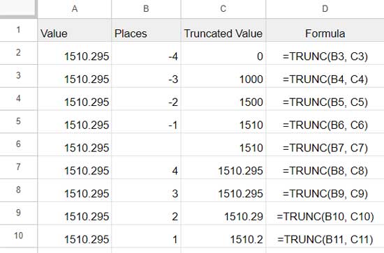
In the given examples, the value to truncate is 1510.295. Let’s explore the TRUNC function using places ranging from -4 to 4 for a clearer understanding.
If the ‘places’ is set to -4, the formula will return 0. It changes 4 digits to the left of the decimal point to 0 and discards all numbers to the right of the decimal point.
=TRUNC(1510.295, -4) // returns 0Specifying -3 as ‘places’ will result in 1000.
=TRUNC(1510.295, -3) // returns 1000To truncate all decimal places except 2, set ‘places’ to 2.
=TRUNC(1510.295, 2) // returns 1510.29If ‘places’ is 0 or unspecified, the formula will truncate all decimal places.
=TRUNC(1510.295) // returns 1510In the following screenshot, ‘values’ and their respective ‘places’ are presented in separate columns (A2:A for ‘values’ and B2:B for ‘places’) to enhance the clarity of the formula.

What about negative values in column A?
The TRUNC function has no issue with negative or positive values. The result will be a positive or negative number based on the sign of the values in column A.
How to Remove Decimal Places in Google Sheets
From the above examples, it’s evident that you can utilize the TRUNC function to eliminate decimal places in Google Sheets. Simply wrap the value with TRUNC as follows:
=TRUNC(value)Example:
=TRUNC(1500.12) // returns 1500Use the following formula if the value is in cell A1:
=TRUNC(A1)Similarly, you can employ the formula to extract the date from a timestamp, as TRUNC will truncate the time component in a datetime value since it’s considered the fractional part.
Difference Between the ROUND and TRUNC Functions in Google Sheets
The only similarity between the ROUND and TRUNC functions lies in their arguments. Both take ‘value’ and ‘places’ arguments.
The ROUND function rounds a ‘value’ to a specific number of decimal ‘places’. Similar to TRUNC, here too, the places can be negative or positive. If negative, the value is rounded at the specified number of digits to the left of the decimal point.
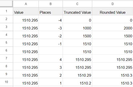
Let’s consider the ‘value’ in cell A3 as 1510.295 and ‘places’ as -3 in cell B3. This is how the TRUNC and ROUND formulas treat these numbers:
=TRUNC(A3, B3) // returns 1000
=ROUND(A3, B3) // returns 2000
If places are set to 2, the formulas will return 1510.29 and 1510.3 respectively. Please refer to the screenshot below for a detailed comparison.

Google Sheets INT Function and Its Difference with TRUNC
Google Sheets INT function returns only the integer part of a number, taking only the ‘value’ argument.
When using TRUNC with only the ‘value’ argument, it also returns the integer part of the number. However, there is a distinction.
The INT function rounds a number down to the nearest integer that is less than or equal to it. The difference becomes apparent when the ‘value’ is a negative number.
For example, if you use -1500.59 within INT, TRUNC, and ROUND, they will return -1501, -1500, and -1501, respectively.
Conclusion
While I have provided comparisons between INT and ROUND with TRUNC, it’s important to emphasize that the primary focus of this tutorial is on the TRUNC function.
The discussions about INT and ROUND are intended to offer a general understanding of their differences from TRUNC. Therefore, your main attention and focus in this tutorial should be directed towards the TRUNC function.
Resources:


TRUNC(Value) and INT(Value) are not actually equivalent. You can see this if you compare the results of INT(-1.5) and TRUNC(-1.5).
INT() will return -2, and TRUNC returns -1. This is because INT will always return the nearest integer which is lower than the value, which causes it to round in a potentially unexpected direction with negative numbers. As opposed to ROUNDDOWN which is basically FLOOR(ABS(Value))*SIGN(Value) and therefore tends to behave like TRUNC.