This article explains how to use nested Query formulas in Google Sheets.
In a nested Query formula, one Query is placed inside another. The result of the subquery (or inner Query) is used as the input for the outer Query. This concept can be challenging to grasp without examples.
Fortunately, I’ve included two examples on this page to help clarify the process.
Before we dive in, if you haven’t checked out my earlier collection of Query tutorials, I recommend searching for the term “Query” on my site.
Let’s get started!
Google Sheets Nested Query
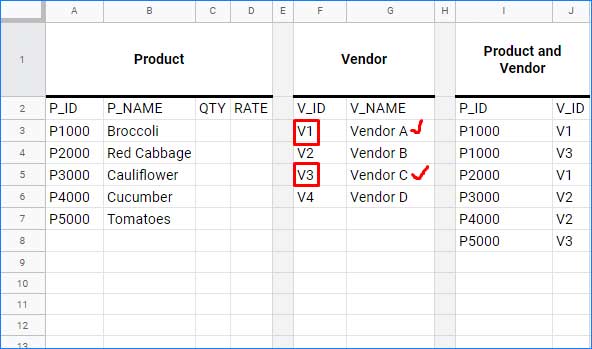
To get started, create three tables in your Google Sheets as shown below. Make sure to follow the specified ranges.
Table 1: Product
Enter the following data in the range A2:D7 on ‘Sheet1’:
| P_ID | P_NAME | QTY | RATE |
| P1000 | Broccoli | ||
| P2000 | Red Cabbage | ||
| P3000 | Cauliflower | ||
| P4000 | Cucumber | ||
| P5000 | Tomatoes |
Table 2: Vendor
Enter the following data in the range F2:G6 on the same sheet:
| V_ID | V_NAME |
| V1 | Vendor A |
| V2 | Vendor B |
| V3 | Vendor C |
| V4 | Vendor D |
Table 3: Product and Vendor
Finally, enter the following data in the range I2:J8 on ‘Sheet1’:
| P_ID | V_ID |
| P1000 | V1 |
| P1000 | V3 |
| P2000 | V1 |
| P3000 | V2 |
| P4000 | V2 |
| P5000 | V3 |
Problems to Solve
I will solve the following two problems using nested Query formulas in Google Sheets:
- Return the Product ID (P_ID) using the Vendor Name (V_NAME).
- Return the Product Name (P_NAME) using the Vendor Name (V_NAME).
To solve these problems, we may need to use an SQL-like IN operator in the Google Sheets nested Query formula.
Before continuing, it’s essential to understand how to use the IN operator in Google Sheets Queries. Let’s dive in!
The Alternative to the SQL IN Operator in Google Sheets Query (Also NOT IN)
Once you understand how to use the IN/NOT IN Query, we can proceed with solving the problems.
SQL Similar IN Operator in Nested Query in Google Sheets
Nested Query Formula with One Subquery
Let’s tackle problem #1: Returning the Product ID (P_ID) using the Vendor Name (V_NAME). This will help identify which products the vendor is selling.
The V_NAME (vendor name) is in Table #2, and the P_ID (product ID) is in Table #3. The common column between these two tables is the V_ID.
First, we’ll filter Table 2 to extract the V_ID (the common field in both tables) from column F that matches “Vendor A” and “Vendor C.”

Subquery Formula:
=QUERY(F3:G, "Select F where G = 'Vendor A' or G = 'Vendor C' ")This subquery formula will return the V_IDs “V1” and “V3.”
Next, we’ll nest this Query formula within another Query formula. Before nesting, let’s test the formulas separately. Now, onto the second formula.
We can filter column I of Table #3 using the V_IDs obtained from the subquery as the criterion.
Without nesting, the formula would look like this, which is also an example of using an SQL-like IN operator in Google Sheets.
Query Formula without Nesting:
=QUERY(I3:J, "Select I where J matches 'V1|V3' ")Assume “V1” is in cell N3 and “V3” is in cell N4. If so, we can rewrite the above query as:
=QUERY(I3:J, "Select I where J matches '"&TEXTJOIN("|", TRUE, N3:N4)&"' ")Now, we can replace N3:N4 with our subquery formula.
Query Formula with Nesting:
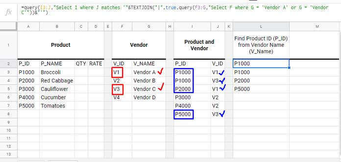
=QUERY(I3:J, "Select I where J matches '"&TEXTJOIN("|", TRUE, QUERY(F3:G, "Select F where G = 'Vendor A' or G = 'Vendor C' "))&"' ")
If you enter it in cell L2, it will return the values P1000, P1000, P2000, and P5000 in the range L2:L5.
The formula above is an example of a nested Query in Google Sheets.
Nested Query Formula with Two Subqueries
Let’s tackle Problem #2: Returning the Product Name (P_NAME) using the Vendor Name (V_NAME). This will help identify which products are associated with the specified vendors.
We want to find the product names supplied by “Vendor A” or “Vendor C.” The vendor names are in Table #2, Product Names are in Table #1. There is no common field in these two tables. So what we will do here is to use our previous formula which returns the Product IDs of the said two vendors and use that to filter the product names in Table #1.
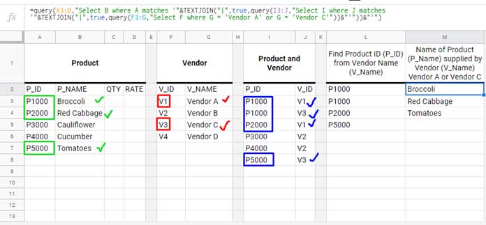
The range L2:L5 contains the Product IDs of the products supplied by “Vendor A” and “Vendor C”. Let’s filter the product names associated with these IDs in Table #1.
Without the subquery, the formula would look like this:
=QUERY(A3:D, "Select B where A matches '"&TEXTJOIN("|", TRUE, L2:L5)&"' ")Here, the range L2:L5 contains the result of the previous Google Sheets nested Query formula.
To incorporate the nested Query, simply replace the range L2:L5 with the nested Query:
=QUERY(A3:D, "Select B where A matches '"&TEXTJOIN("|", TRUE, QUERY(I3:J, "Select I where J matches '"&TEXTJOIN("|", TRUE, QUERY(F3:G,"Select F where G = 'Vendor A' or G = 'Vendor C'"))&"' "))&"' ")
I’ve done my best to explain the usage of nested Queries in Google Sheets. If you have any questions or notice any errors, please let me know.
Additional Notes
In some cases, such as solving Problems 1 and 2 above, there is no need to use nested Queries in Google Sheets.
As an alternative, you can use VLOOKUP or sometimes a reverse VLOOKUP (in a nested form) instead of subqueries or nested Queries.
We will discuss this approach in a separate tutorial later.
Note: When nesting Queries, please be mindful of the proper use of Query literals.


U are a gem.
Flipping Genius, Thanks!!!