


")


")

")
")
 in Excel & Google Sheets")


Google Sheets allows you to highlight an entire column if any cell has an error, making it easy to spot and fix issues in your data. In this tutorial, you’ll learn how to use conditional formatting with a custom formula to automatically highlight columns that contain errors like #DIV/0! or #VALUE!.
Why Highlight an Entire Column Instead of Just the Error Cells?
Highlighting an entire column instead of just the specific error cells has its benefits.
Imagine you have a large dataset with numeric columns, and the total for each column is calculated at the bottom. If any cell in a column contains an error, the total will also return an error. Instead of scrolling down to check whether the total is incorrect, you can immediately identify problematic columns by highlighting the entire column containing errors.
You can apply this formatting to a single column or all columns in a range. When applied to multiple columns, it becomes easier to locate and investigate columns with errors.
Google Sheets Doesn’t Have a Built-in Rule for This—Here’s the Solution
Google Sheets doesn’t offer a built-in rule to highlight an entire column if any cell in that column contains an error. Instead, you need to use a custom formula, and that’s where I can help.
Custom Formula for Highlighting an Entire Column
Use the following formula in conditional formatting:
=ArrayFormula(XMATCH(TRUE, ISERROR(range)))rangerefers to the column you want to highlight.- The row reference should be absolute, while the column reference should be relative to ensure the rule applies correctly.
Let’s go through an example to see this in action.
Step 1: Setting Up the Sample Data
Here’s a sample dataset:
| Product | Price | Quantity | Total |
| Apple | 1.5 | 10 | 15 |
| Banana | 0.75 | 8 | 6 |
| Cherry | 2 | 10 | #DIV/0! |
| Date | 1.25 | 5 | 6.25 |
| Elderberry | #VALUE! | 3 | #VALUE! |
| Fig | 2.5 | 4 | 10 |
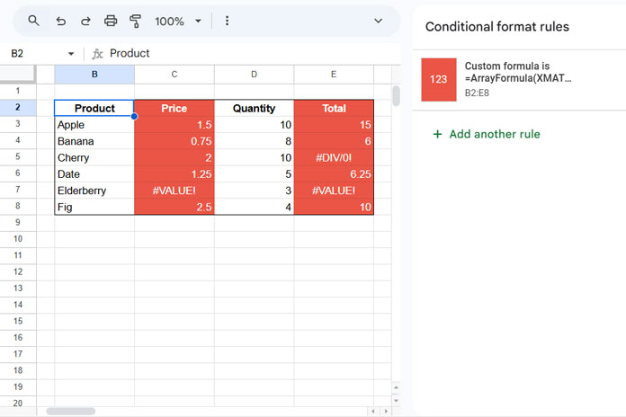
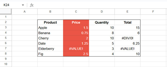
This data is arranged in B2:E8 in my sheet. You can use the same range for testing. If you’re applying this to your own dataset, I’ll explain what adjustments you need to make.
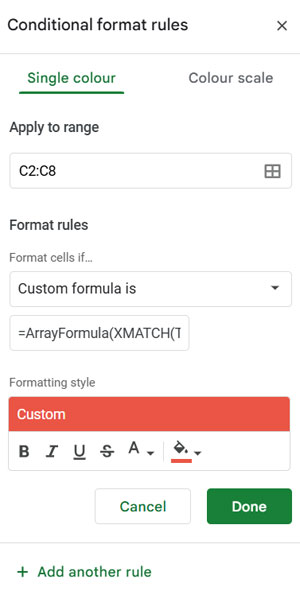
Step 2: Selecting the Column for Conditional Formatting
We’ll first apply the rule to column C (C2:C8) to see how to highlight the entire column if any cell contains an error. In this dataset, C7 contains a #VALUE! error, so the rule should highlight the whole column.
Step 3: Applying the Conditional Formatting Rule
- Select C2:C8 (or the column range you want to highlight).
- Click Format > Conditional formatting to open the Conditional format rules panel
- Under Format rules, select Custom formula is
- Enter the formula:
=ArrayFormula(XMATCH(TRUE, ISERROR(C$2:C$8)))
(ReplaceC$2:C$8with the range of the column you want to highlight.) - Under Formatting style, choose a fill color (e.g., red)
- Click Done
Now, if any cell in C2:C8 contains an error, the entire column will be highlighted.
Bonus: Expanding to Multiple Columns
If you want to apply this rule to the entire table (B2:E8), follow these steps:
- Select B2:E8 instead of C2:C8.
- Use the modified formula:
=ArrayFormula(XMATCH(TRUE, ISERROR(B$2:B$8)))
This will highlight entire columns in the selected range if any cell in that column contains an error.
How the Formula Works
ISERROR(B$2:B$8): Returns an array of TRUE or FALSE, where TRUE indicates an error.XMATCH(TRUE, ISERROR(B$2:B$8)): Finds the position of the first error in the column. If an error is found, the column is highlighted.- Since the row reference is absolute (
$2:$8), and the column reference is relative (B$2:B$8), the formula dynamically applies to each column in the selected range.