FIND Function in Google Sheets

The FIND function is a case-sensitive function that returns the position at which a string is first found within a text in Google Sheets.

There is a similar function called SEARCH, which is more commonly used because it’s case-insensitive.

Similar to SEARCH, the FIND function is often used in combination with MID or for filtering rows based on partial matches.

Table of Contents

Find Function: Syntax and Arguments

Syntax:

FIND(search_for, text_to_search, [starting_at])

Arguments:

search_for: The string to find within text_to_search.
text_to_search: The text or the cell reference containing the text in which to search for the first occurrence of search_for.
starting_at (optional): The character’s position within text_to_search at which to start the search.

Example:

=FIND("USD", "Pay USD 1,200.00") // returns 5
=FIND("usd", "Pay USD 1,200.00") // returns #VALUE error

To handle the error, use the IFERROR function:

=IFERROR(FIND("usd", "Pay USD 1,200.00"))

The starting_at argument requires thorough understanding to avoid errors. Please see the following formulas:

=FIND(" ", "01 123456789 123", 1)
=FIND(" ", "01 123456789 123", 2)
=FIND(" ", "01 123456789 123", 3)

All these formulas will return 3 even though the starting_at is different. This is because, when returning the position, the FIND function starts the count from the first character, not from starting_at.

The following formula returns 13 since starting_at is 4 and the first space character after this starting_at is the 13th character. Here also, the count starts from the very first character in the text:

=FIND(" ", "01 123456789 123", 4)

Using the FIND Function as a FILTER Condition in Google Sheets

The FILTER function does not support wildcards in Google Sheets. Therefore, to filter rows based on partial text matches within a column, you can use FIND or SEARCH functions. Note that FIND is case-sensitive, whereas SEARCH is not.

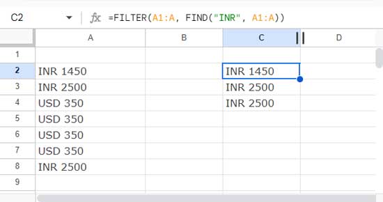
=FILTER(A1:A, FIND("INR", A1:A))

FIND function with FILTER function in Google Sheets

The above combination of FILTER and FIND functions filters rows where the value contains “INR”.

For more advanced pattern matching, consider using REGEXMATCH instead of FIND in Google Sheets.

MID and FIND Combo

Here is an interesting combination of MID and FIND functions in Google Sheets.

Cell A1 contains the following text:

After a long day at work, Mr. Ben relaxed with a good book

In cell B1, you can use the formula to extract the name “Ben”:

=LET(mr, FIND("Mr. ", A1)+4, fs, FIND(" ", A1, mr), n, fs-mr, MID(A1, mr, n))

FIND("Mr. ", A1) + 4 returns the starting point of the name in the text (named ‘mr’).
FIND(" ", A1, mr) returns the starting point of the text after the name (named ‘fs’).
fs - mr returns the number of characters in the name.
The MID formula, MID(A1, mr, n), returns the text starting at ‘mr’ and extracts ‘n’ characters.

If you understand this formula, you will become a proficient user of the FIND function.