


")


")

")
")
 in Excel & Google Sheets")


Comparing two tables and removing duplicates in Google Sheets means identifying rows or data that exist in both tables and eliminating them from one of the tables.
For example, consider the following data in Sheet1, range A1:B:
| Name | Age |
| Rose | 25 |
| Bob | 30 |
| Mike | 35 |
| Ben | 25 |
And this data in Sheet2, range A1:B:
| Name | Age |
| Rose | 25 |
| David | 40 |
| Mike | 35 |
Let’s compare these two tables and remove duplicates. You can decide from which table you want to remove duplicates.
- If you consider Table1, you’ll retain rows with “Bob” and “Ben” after removing duplicates.
- If you consider Table2, you’ll retain the row with “David.”
Below, I’ll provide the formula for Sheet1 and explain the adjustments you should make to apply it to Sheet2 instead.
Step 1: Compare Two Tables and Identify Duplicates
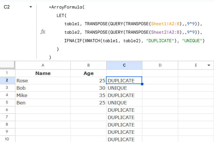
In cell C2 of Sheet1, enter the following formula:
=ArrayFormula(
   LET(
      table1, TRANSPOSE(QUERY(TRANSPOSE(Sheet1!A2:B),,9^9)),
      table2, TRANSPOSE(QUERY(TRANSPOSE(Sheet2!A2:B),,9^9)),
      IFNA(IF(XMATCH(table1, table2), "DUPLICATE"), "UNIQUE")
   )
)
This formula will return “DUPLICATE” for duplicate rows and “UNIQUE” for others.
Formula Breakdown:
TRANSPOSE(QUERY(TRANSPOSE(Sheet1!A2:B), , 9^9))- Converts multiple columns in Sheet1 (range A2:B) into a single-column format for easy comparison. This approach is versatile and works well for combining data from multiple columns. You can read more about this functionality in A Flexible Array Formula for Joining Columns in Google Sheets.
TRANSPOSE(QUERY(TRANSPOSE(Sheet2!A2:B), , 9^9))- Converts multiple columns in Sheet2 (range
A2:B) into a single-column format.
- Converts multiple columns in Sheet2 (range
LET(table1, ..., table2, ...)- Assigns these results to
table1andtable2, allowing for cleaner and reusable references in the formula.
- Assigns these results to
XMATCH(table1, table2)- Matches
table1values withtable2. Returns a number for matches and an error (#N/A) for non-matches.
- Matches
IFNA(IF(..., "DUPLICATE"), "UNIQUE")- Labels matches as “DUPLICATE” and non-matches as “UNIQUE.”
This step identifies duplicates between the two tables. Now let’s proceed to remove them.
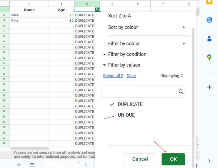
Step 2: Filter and Remove Duplicates
- Select column C.
- Click Data > Create a Filter.
- Click the dropdown arrow in cell C1 and uncheck “UNIQUE.”
- Click OK to filter out unique rows.
- Select the remaining rows (excluding the header).
- Click Edit > Delete Rows.
- Turn off the filter by clicking Data > Remove Filter.
Modifications to Apply the Formula in Sheet2
If you want to apply the formula in Sheet2 instead of Sheet1, make the following change:
Replace XMATCH(table1, table2) with XMATCH(table2, table1). The updated formula becomes:
=ArrayFormula(
   LET(
      table1, TRANSPOSE(QUERY(TRANSPOSE(Sheet1!A2:B),,9^9)),
      table2, TRANSPOSE(QUERY(TRANSPOSE(Sheet2!A2:B),,9^9)),
      IFNA(IF(XMATCH(table2, table1), "DUPLICATE"), "UNIQUE")
   )
)
Enter this formula in cell C2 of Sheet2 and follow the same filtering process described above.
Conclusion
This method provides a flexible approach to compare two tables and remove duplicates. If your data spans multiple columns and you want to compare only specific columns, adjust the formula ranges accordingly.
For example:
- To compare only columns
A:Cin both sheets (if the data spansA:Z), useSheet1!A1:CandSheet2!A1:Cin the formula. - For non-adjacent columns like
A,D, andF, combine them with HSTACK, e.g.,HSTACK(Sheet1!A1:A, Sheet1!D1:D, Sheet1!F1:F).