The replacement for the CONCAT function in Google Sheets is the ampersand operator, not CONCATENATE, JOIN, or TEXTJOIN.
The key distinction of the CONCAT function from the other three text join functions is its ability to expand using ARRAYFORMULA into multiple cells.
The other three require the assistance of Lambda Helper functions for expansion, making them more complex. However, they each have their specialties.
In this guide, we will explore how to use the CONCAT function in Google Sheets and also demonstrate its usage in nested forms.
I’ve already mentioned that this function replaces the ampersand operator. So, if you use multiple ampersand operators to join texts, you might want to use multiple CONCATs. In that case, we employ a nested approach.
Syntax and Arguments
Syntax:
CONCAT(value1, value2)Arguments:
value1: The value (text, number, date, time, or timestamp) to whichvalue2will be appended.value2: The value to append tovalue1.
If either value1 or value2, or both, are arrays, you must input the formula as an array formula.
Basic Examples of CONCAT Function in Google Sheets
Formula 1:
=CONCAT("ABC", 123) // returns the string "ABC123"The equivalent of the above formula is:
="ABC"&123Here are two examples of CONCAT array formulas:
Formula 2:
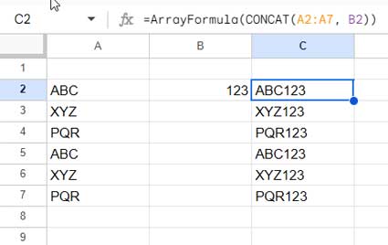
=ArrayFormula(CONCAT(A2:A7, B2))
=ArrayFormula(A2:A7 & B2)
The above formula produces an array of concatenated values, where each element is the concatenation of the corresponding cell in column A with the value in cell B2.
Formula 3:
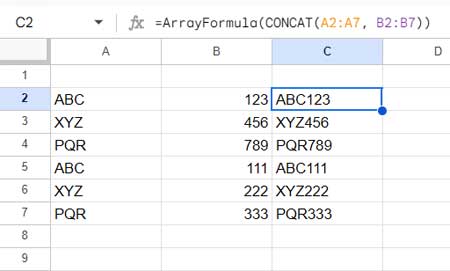
=ArrayFormula(CONCAT(A2:A7, B2:B7))
=ArrayFormula(A2:A7 & B2:B7)
This formula produces an array of concatenated values, where each element is the concatenation of the corresponding cell in column A with the corresponding cell in column B.

Note:
When using the CONCAT function in an array formula, the value1 and value2 must be of equal size, or either can be a single value. Otherwise, the formula may return errors in some cells.
Nested CONCAT: Text Strings
In the following real-life example of combining text with text, we are merging titles with names. This can expedite your data entry, especially if you opt to use this within an array formula.
To combine two texts in Google Sheets, simply use the “&” operator between the texts or employ the CONCAT function in Google Sheets.
If you want to include a space between the concatenated texts, you may use nested CONCAT, as demonstrated in the examples below.
| A | B | C | D | |
| 1 | Title | Name | Formula | Result |
| 2 | Mr. | Johnson | =A2&" "&B2=CONCAT(CONCAT(A2, " "), B2) | Mr. Johnson |
| 3 | Mr. | Arun | =A3&" "&B3=CONCAT(CONCAT(A3, " "), B3) | Mr. Arun |
| 4 | Ms. | Elina | =A4&" "&B4=CONCAT(CONCAT(A4, " "), B4) | Ms. Elina |
Let me explain the first nested CONCAT formula in cell C2 so that you can understand the rest of them.
Formula:
=CONCAT(CONCAT(A2, " "), B2Explanation:
CONCAT (A2, " "): This inner CONCAT function combines the title in cell A2 with a space character. So, it concatenates “Mr.” with a space, resulting in “Mr. “.
CONCAT(..., B2): The outer CONCAT function then combines the result from the inner CONCAT with the name in cell B2. It concatenates “Mr. ” with “John”, producing the final output “Mr. John”.
Can we use nested CONCAT functions in an array formula in Google Sheets?
Yes, similar to the ampersand, we can use nested CONCAT in array formulas. In the above examples, you can replace the formulas in cells C2:C4 with either of the following array formulas in cell C2:
=ArrayFormula(A2:A4&" "&B2:B4)
=ArrayFormula(CONCAT(CONCAT(A2:A4, " "), B2:B4))
Nested CONCAT: Text and Number
To combine a number with text, we can use either the CONCAT or ampersand. Here also, we will apply the nested CONCAT.
When you have formatted numbers, such as currency, you may need to use the TEXT function with the CONCAT function. Please see cell C5 for an example.
| A | B | C | D | |
| 1 | Product ID_I | Product ID_II | Formula | Result |
| 2 | 25011 | AX | =A2&" "&B2=CONCAT(CONCAT(A2, " "), B2) | 25011 AX |
| 3 | 25012 | AZ | =A3&" "&B3=CONCAT(CONCAT(A3, " "), B3) | 25012 AZ |
| 4 | Bill Value | Text | Formula | Result |
| 5 | 150.25 | Amount: | =B5&" "&TEXT(A5, "$#,##0.00")=CONCAT(CONCAT(B5, " "), TEXT(A5, "$#,##0.00")) | Amount: $150.25 |
Nested CONCAT: Text and Date
Below, we have student names in column A, and their DOB in column B. Let’s see how to combine them using the CONCAT (nested) function in Google Sheets.
When concatenating text with a date using CONCAT, you should use the TEXT function. Otherwise, the formula will convert the date to date values. This is because a date is essentially a number formatted as a date in Google Sheets.
| A | B | C | D | |
| 1 | Name | DOB | Formula | Result |
| 2 | Emily | 23/11/2009 | =A2&"'s"&" DOB is "&TEXT(B2, "dd/mm/yyyy")=CONCAT(CONCAT(CONCAT(A2, "'s")," DOB is "), TEXT(B2, "dd/mm/yyyy")) | Emily’s DOB is 23/11/2009 |
| 3 | Liam | 26/03/2009 | =A3&"'s"&" D.O.B. is "&TEXT(B3, "dd/mm/yyyy")=CONCAT(CONCAT(CONCAT(A3, "'s"), " DOB is "), TEXT(B3,"dd/mm/yyyy")) | Liam’s DOB is 26/03/2009 |
| 4 | Isabella | 31/03/2009 | =A4&"'s"&" D.O.B. is "&TEXT(B4, "dd/mm/yyyy")=CONCAT(CONCAT(CONCAT(A4, "'s"), " DOB is "), TEXT(B4,"dd/mm/yyyy")) | Isabella’s DOB is 31/03/2009 |
| 5 | Text | Date | Formula | Result |
| 6 | Today is | =TODAY() | =A6&" "&TEXT(B6, "dd/mm/yyyy")=CONCAT(CONCAT(A6, " "), TEXT(B6, "dd/mm/yyyy")) | Today is 13/01/2024 |
CONCAT Function for Combining Text and Timestamp in Google Sheets
See how to concatenate date-time/timestamp with text.
When combining time with text, you can use either the 12-hour (AM/PM) or the 24-hour format. I am combining the date-time “20/07/2018 23:43:44” in cell A1 with the text “recorded date and time is”:
="Recorded date-time is "&TEXT(A1,"DD/MM/YYYY HH:MM:SS AM/PM")The same using the Google Sheets CONCAT function:
=CONCAT("Recorded date-time is ",TEXT(A1,"DD/MM/YYYY HH:MM:SS AM/PM"))Result: “Recorded date-time is 20/07/2018 11:43:44 pm.”
If you remove the highlighted part, i.e., AM/PM, from the formulas, the time will be in the 24-hour format.
Resources
- Combine Text and Date in a Google Docs Spreadsheet Using Formula.
- Difference Between JOIN, TEXTJOIN, and CONCATENATE Functions in Google Sheets.
- The Flexible Array Formula to Join Columns in Google Sheets.
- How to Concatenate a Number without Losing Its Format in Google Sheets.
- Concatenate Double Quotes with Text in Google Sheets.
- Concatenate Two, Three, or More Than Three Columns in Google Sheets.
- How to Properly Concatenate Start Time with End Time in Google Sheets.


