Get the Latest Non-Blank Value by Date in Google Sheets

There’s no built-in function in Google Sheets to retrieve the latest non-blank value by date—but you can achieve it using a custom formula made with native functions.

When working with multiple records (rows) related to a specific category (like a user or item), you may want to find the latest non-blank value among them based on date.

Table of Contents

Real-Life Example

Let’s say you bought 1 liter of cooking oil on 25/07/2023, 06/08/2023, and 23/08/2023, with prices recorded as $3.52, $4.00, and blank (because you lost the bill).

In this case, the most recent price should not return a blank cell. Instead, it should return $4.00, the last known price.

This issue commonly occurs when using Google Forms to collect data into Google Sheets. For instance, a user might resubmit a form to update previously entered data.

These types of datasets typically include:

A date or timestamp column
A category column
A values column (which may have blanks)

To look up the latest non-blank value by date in Google Sheets, we can use a combination of the FILTER, SORT, and VLOOKUP functions—or build a more advanced array formula.

Example: Get the Latest Non-Blank Value by Date in Google Sheets

Consider a table with three columns:

Measured Date (A)
Breed (B)
Height in Inches (C)

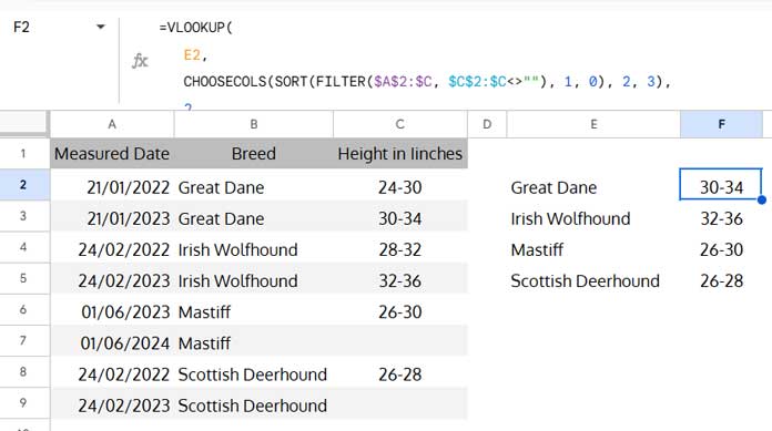
Measured Date	Breed	Height in Iinches
21/01/2022	Great Dane	24-30
21/01/2023	Great Dane	30-34
24/02/2022	Irish Wolfhound	28-32
24/02/2023	Irish Wolfhound	32-36
01/06/2023	Mastiff	26-30
01/06/2024	Mastiff
24/02/2022	Scottish Deerhound	26-28
24/02/2023	Scottish Deerhound

To return the latest non-blank height per dog breed, enter this formula in cell F2:

=VLOOKUP(
   E2, 
   CHOOSECOLS(SORT(FILTER($A$2:$C, $C$2:$C<>""), 1, 0), 2, 3), 
   2, 
   FALSE
)

Then drag it down to apply to other breeds in the column.

Example showing how to get the latest non-blank value by date in Google Sheets using a formula

Array Formula Version

To return values for multiple breeds at once, use:

=ArrayFormula(
   VLOOKUP(
      E2:E5, 
      CHOOSECOLS(SORT(FILTER(A2:C, C2:C<>""), 1, 0), 2, 3), 
      2, 
      FALSE
   )
)

This array formula returns the latest non-blank value by date in Google Sheets, specifically from the “Height in Inches” column, for each breed in the criteria range.

Formula Breakdown

Let’s understand how this formula works:

FILTER(A2:C, C2:C<>""): Filters out rows where the value column (height) is blank.
SORT(..., 1, 0): Sorts the filtered data in descending order by the date in column A (latest dates first).
CHOOSECOLS(..., 2, 3): Rearranges columns so that VLOOKUP works correctly, making column B (Breed) the lookup column and column C (Height) the return column.
VLOOKUP(E2, ..., 2, FALSE): Looks up the breed from cell E2 and returns the height from the most recent non-blank entry.

Notes

E2 or E2:E5: Criteria range (breeds to look up)
A2:C: The dataset range
C2:C: The column from which we want the latest non-blank value (height)

Your dataset may vary, so understanding the logic behind the formula will help you adapt it to different scenarios.